TRANSPORT
This keyword data block is
used to simulate one-dimensional (1D) transport of solutes, water, colloids,
and heat due to the processes of advection and dispersion, diffusion, and
diffusion into stagnant zones adjacent to the 1D flow system. Radial and three-dimensional
(3D) diffusion can be modeled by using stagnant zones. Multicomponent diffusion
allows individual tracer diffusion coefficients to be used in calculating the
diffusion of ions; TRANSPORT has capabilities to model
multicomponent diffusion in the aqueous solution and in the interlayers of
swelling clay minerals. All the chemical processes modeled by PHREEQC,
including kinetically controlled reactions, may be included in an
advective-dispersive transport simulation. Purely advective transport plus
reactions--without diffusion, dispersion, or stagnant zones--can be simulated
with the ADVECTION data block.
Example data block
Line 0: TRANSPORT
Line 1: -cells 5
Line 2: -shifts 25
Line 3: -time_step 1 yr 2.0
Line 4: -flow_direction forward
Line 5: -boundary_conditions flux constant
Line 6: -lengths 4*1.0 2.0
Line 7: -dispersivities 4*0.1 0.2
Line 8: -correct_disp true
Line 9: -diffusion_coefficient 1.0e-9
Line 10: -stagnant 1 6.8e-6 0.3 0.1
Line 11: -thermal_diffusion 3.0 0.5e-6
Line 12: -initial_time 1000
Line 13: -print_cells 1-3 5
Line 14: -print_frequency 5
Line 15: -punch_cells 2-5
Line 16: -punch_frequency 5
Line 17: -dump dump.file
Line 18: -dump_frequency 10
Line 19: -dump_restart 20
Line 20: -warnings false
Line 21: -multi_D true 1e-9 0.3 0.05 1.0 true
Line 22: -interlayer_D true 0.09 0.01 250
Line 23: -porosities 4*0.3 0.25
Line 24: -current 1e-3
Line 25: -implicit true 1.0 -30
Line 26: -same_model 2-5 8-11
Explanation
TRANSPORT is the
keyword for the data block. No other data are input on the keyword line.
-cells --Indicates the number of
cells in the 1D column for the advective-dispersive transport simulation.
Optionally, cells or -c [ ells ].
cells --Number of cells in a 1D
column. Default is 1.
-shifts --Indicates the number of
shifts or diffusion periods in the advective-dispersive transport simulation.
Optionally, shifts or -s [ hifts ].
shifts --For advective-dispersive
transport, shifts is the number of advective
shifts or time steps, which is the number of times the solution in each cell
will be shifted to the next higher or lower numbered cell; the total time
simulated is ![]() . For purely diffusive transport, shifts is the number of diffusion periods that are simulated; the
total diffusion time is
. For purely diffusive transport, shifts is the number of diffusion periods that are simulated; the
total diffusion time is ![]() . Default is 1.
. Default is 1.
Line 3: -time_step time_step [unit] [substeps]
-time_step --Defines time step associated with each advective shift or
diffusion period. The number of shifts or diffusion periods is given by -shifts .
Optionally, timest , -t [ imest
], time_step , or -t
[ ime_step ].
time_step --Time (second) associated with each shift or diffusion period.
Default is 0 s.
unit --Optional time unit may be second , minute , hour
, day , year , or an abbreviation of one of
these units. The time_step is converted to seconds
after reading the data block; all internal calculations, Basic functions, and
output times are in seconds. Default is second.
substeps--
Subdivides the time step into substeps intervals.
Used only in multicomponent diffusion calculations, where time_step
reduction can help to avoid negative concentrations. The negative
concentrations may occur when the time step is too large relative to the
explicitly defined stagnant-cell mixing factors; too large a time step causes
the Von Neumann criterion to be violated. Default is 1.
Line 4: -flow_direction ( forward , back , or diffusion_only )
-flow_direction --Defines direction of flow. Default is forward at
startup. Optionally, direction , flow
, flow_direction , -dir [ ection
], or -f [ low_direction
].
forward , back , or diffusion_only
--(1) Forward , advective flow direction is into higher
numbered cells; optionally, f [ orward
], (2) Backward , advective flow direction is into lower
numbered cells; optionally b [ ackward
], or (3) Diffusion_only , only
diffusion occurs, there is no advective flow; optionally d [
iffusion_only ] or n [
o_flow ].
Line 5: -boundary_conditions first,
last
-boundary_conditions --Defines boundary conditions for the first and last cell.
Optionally, bc , bcond ,
-b [ cond ], boundary_condition , -b [
oundary_condition ]. Three types of boundary
conditions are allowed at either end of the column (indicated by ![]() ):
):
constant --Concentration is constant ![]() , also known
as first type or Dirichlet boundary condition. C 0 is the
concentration outside the column (mol/kgw).
Optionally, co [ nstant ] or 1 .
, also known
as first type or Dirichlet boundary condition. C 0 is the
concentration outside the column (mol/kgw).
Optionally, co [ nstant ] or 1 .
closed --No flux at boundary, v = 0
and ![]() , also known
as second type or Neumann boundary condition, where v is the flow velocity
(m/s, meter per second). Optionally, cl [ osed ]
or 2 .
, also known
as second type or Neumann boundary condition, where v is the flow velocity
(m/s, meter per second). Optionally, cl [ osed ]
or 2 .
flux --Flux
boundary condition, ![]() , also known as third type or Cauchy boundary condition, where DL
is the dispersion coefficient (m2/s). Optionally, f [ lux ] or 3
.
, also known as third type or Cauchy boundary condition, where DL
is the dispersion coefficient (m2/s). Optionally, f [ lux ] or 3
.
first --Boundary condition at the
first cell, constant , closed
, or flux . Default is flux
.
last --Boundary condition at the
last cell, constant , closed
, or flux . Default is flux
.
Line 6: -lengths list of lengths
-lengths --Defines length of each
cell for advective-dispersive transport simulations (m). Optionally, length , lengths , or -l
[ engths ].
list of lengths --Length
of each cell (m). Any number of lengths up to the total number of
cells ( cells ) may be entered. If cells
is greater than the number of lengths
entered, the final value read will be used for the remaining cells. Multiple
lines may be used. Repeat factors can be used to input multiple data with the
same value; in the Example data block, 4*1.0 is interpreted as 4 values of 1.0.
Default is 1 m.
Line 7: -dispersivities list
of dispersivities
-dispersivities --Defines dispersivity of each cell for
advective-dispersive transport simulations (m). Optionally, disp , dispersivity , dispersivities
, -dis [ persivity
], or -dis [ persivities
].
list of dispersivities --Dispersivity assigned to each cell
(m). Any number of dispersivities up to the
total number of cells ( cells ) may be
entered. If cells is greater than the number
of dispersivities entered, the final value
read will be used for the remaining cells. Multiple lines may be used. Repeat
factors can be used to input multiple data with the same value; in the Example
data block, 4*0.1 is interpreted as 4 values of 0.1 m. Default is 0 m.
Line 8: -correct_disp [( True or False )]
-correct_disp --Dispersivity is multiplied by (1 + 1/
cells )
for column ends with flux boundary conditions. This correction can improve
modeling effluent composition from column experiments that are modeled with few
cells. Default is false at startup. Optionally, correct_disp or -co [
rrect_disp ].
( True or False
)-- True indicates that dispersivity
is corrected for flux-boundary end cells; false indicates that
no correction is made. If neither true nor false
is entered on the line, true is assumed. Optionally, t [ rue ] or f [
alse ].
Line 9: -diffusion_coefficient diffusion coefficient
-diffusion_coefficient --Defines diffusion coefficient for all aqueous species (m 2
/s) when not using multicomponent diffusion ( -multi_D false ); this
value of the diffusion coefficient is also used as the default thermal
diffusion coefficient (see -thermal_diffusion
). Default is 0.3 × 10 -9 m 2 /s at startup.
Optionally, diffusion_coefficient , diffc , -dif [ fusion_coefficient
], or -dif [ fc ].
diffusion coefficient --Diffusion coefficient.
Line 10: -stagnant
stagnant_cells [ exchange_factor ![]()
![]() ]
]
-stagnant --Defines
the maximum number of stagnant (immobile) cells associated with each cell in
which advection occurs (mobile cell). Each mobile cell may be
connected with up to stagnant_cells
immobile cells. The immobile cells associated with a mobile cell are
usually conceived to be a 1D column of cells in which solutes from the mobile
cell diffuse laterally. However, the connections among the immobile cells can
be defined freely with MIX data
blocks, which allows calculation of multidimensional diffusion processes
(Appelo and Wersin, 2007) and radial diffusion (Appelo and others, 2008, see See Modeling
Diffusion of HTO, 36Cl-, 22Na+, and Cs+ in a Radial Diffusion Cell). The
immobile cells associated with a mobile cell, cell ,
are numbered as follows: ![]() , where cells is the number of mobile cells and
, where cells is the number of mobile cells and ![]() . For each
immobile cell, a solution (SOLUTION,
SOLUTION_SPREAD, or SAVE data block) must be defined, and
either a MIX data block or, for
the first-order exchange model, the exchange_factor
must be defined (only applicable if stagnant_cells
equals 1). Mixing will be performed at each diffusion/dispersion time step. EQUILIBRIUM_PHASES, EXCHANGE, GAS_PHASE, KINETICS, REACTION, REACTION_TEMPERATURE, SOLID_SOLUTIONS, and SURFACE may be defined for an
immobile cell. Thermal diffusion in excess of
hydrodynamic diffusion can be calculated only for the first-order exchange
model. Optionally, stagnant or -st
[ agnant ].
. For each
immobile cell, a solution (SOLUTION,
SOLUTION_SPREAD, or SAVE data block) must be defined, and
either a MIX data block or, for
the first-order exchange model, the exchange_factor
must be defined (only applicable if stagnant_cells
equals 1). Mixing will be performed at each diffusion/dispersion time step. EQUILIBRIUM_PHASES, EXCHANGE, GAS_PHASE, KINETICS, REACTION, REACTION_TEMPERATURE, SOLID_SOLUTIONS, and SURFACE may be defined for an
immobile cell. Thermal diffusion in excess of
hydrodynamic diffusion can be calculated only for the first-order exchange
model. Optionally, stagnant or -st
[ agnant ].
stagnant_cells --Maximum number of stagnant (immobile) cells associated with a
mobile cell. Default is 0.
exchange_factor --Factor describing exchange between a mobile and its immobile
cell (s -1 ).
The exchange_factor can be used only if stagnant_cells is 1, in which case all immobile
cells have the same diffusion properties. WARNING: If exchange_factor
is entered, all previously defined MIX structures will be
deleted and MIX structures for the first-order exchange model
for a dual porosity medium will be created. Default is 0 s -1 .
![]() --Porosity in each mobile cell, expressed as a fraction of the
total volume of mobile and immobile cells. The
--Porosity in each mobile cell, expressed as a fraction of the
total volume of mobile and immobile cells. The ![]() is used
only if stagnant_cells is
1, in which case all mobile cells have the same porosity. Default is 0
(unitless).
is used
only if stagnant_cells is
1, in which case all mobile cells have the same porosity. Default is 0
(unitless).
![]() --Porosity in each immobile cell, expressed as a fraction of the
total volume of mobile and immobile cells. The
--Porosity in each immobile cell, expressed as a fraction of the
total volume of mobile and immobile cells. The ![]() is used only
if stagnant_cells is
1, in which case all immobile cells have the same porosity. Default is 0
(unitless).
is used only
if stagnant_cells is
1, in which case all immobile cells have the same porosity. Default is 0
(unitless).
Line 11: -thermal_diffusion
temperature retardation factor, thermal diffusion coefficient
-thermal_diffusion --Defines parameters for calculating the diffusive part of heat
transport. Diffusive heat transport will be calculated as a separate process if
the temperature in any of the solutions of the transport domain differs by more
than 1 °C, and when the thermal diffusion coefficient is larger than
the effective (aqueous) diffusion coefficient . Otherwise, diffusive heat
transport is calculated as a part of aqueous diffusion. The temperature
retardation factor ,
R T , is defined as the ratio of the heat capacity of the total
aquifer over the heat capacity of water in the pores, ![]() , where
, where ![]() is the water filled porosity,
is the water filled porosity,
![]() is density
(kg/m 3 , kilogram per cubic meter), k is specific heat (kJ°C -1 kg -1 ), and subscripts w
and s indicate water and solid, respectively. The thermal diffusion
coefficient,
is density
(kg/m 3 , kilogram per cubic meter), k is specific heat (kJ°C -1 kg -1 ), and subscripts w
and s indicate water and solid, respectively. The thermal diffusion
coefficient, ![]() , can be estimated by using
, can be estimated by using ![]() , where
, where ![]() is the heat conductivity of the aquifer, including pore water and
solid (kJ°C -1 m -1 s -1 ,
kilojoule per degree Celsius, per meter per second). The value of
is the heat conductivity of the aquifer, including pore water and
solid (kJ°C -1 m -1 s -1 ,
kilojoule per degree Celsius, per meter per second). The value of ![]() may be 100 to 1500 times
larger than the aqueous diffusion coefficient, or about 1 × 10 -6
m 2 /s. A temperature change during transport is reduced by the
temperature retardation factor (unitless) to account for the heat capacity of
the matrix. Optionally, -th [
ermal_diffusion ].
may be 100 to 1500 times
larger than the aqueous diffusion coefficient, or about 1 × 10 -6
m 2 /s. A temperature change during transport is reduced by the
temperature retardation factor (unitless) to account for the heat capacity of
the matrix. Optionally, -th [
ermal_diffusion ].
temperature retardation factor
--Temperature retardation factor, unitless. Default is 2.0 (unitless).
thermal diffusion coefficient --Thermal
diffusion coefficient. Default is the aqueous diffusion coefficient.
Line 12: -initial_time initial_time
-initial_time --Identifier to set the time at the beginning of a transport simulation.
The identifier sets the initial value of the variable controlled by -time
in the SELECTED_OUTPUT data block.
Optionally, initial_time or -i [ nitial_time ].
initial_time --Time (seconds) at the beginning of the transport simulation.
Default is the cumulative time including all preceding ADVECTION simulations (for which -time_step has been defined) and all preceding TRANSPORT simulations.
Line 13: -print_cells list
of cell numbers
-print_cells --Identifier to select cells for which results will be written to
the output file. Optionally, print , print_cells , or -pr [
int_cells ]. Note that the hyphen is
required to avoid a conflict with the keyword PRINT.
list of cell numbers --Printing
to the output file will occur only for these cell numbers. The list of cell
numbers may be continued on the succeeding line(s). A range of cell numbers may
be included in the list in the form m-n , where m and n
are positive integers, m is less than n , and the two numbers
are separated by a hyphen without intervening spaces. Default is 1- cells .
Line 14: -print_frequency print_modulus
-print_frequency --Identifier to select shifts for which results will be written
to the output file. Optionally, print_frequency , -print_f [ requency
], output_frequency , or -o
[ utput_frequency ].
print_modulus --Printing to the output file will occur for advection shifts or
diffusion periods that are evenly divisible by print_modulus . Default is 1.
Line 15: -punch_cells list
of cell numbers
-punch_cells --Identifier to select cells for which results will be written to
the selected-output file. Optionally, punch
, punch_cells , -pu [ nch_cells
], selected_cells , or -selected_c [ ells ].
list of cell numbers --Printing
to the selected-output file will occur only for these cell numbers. The list of
cell numbers may be continued on the succeeding line(s). A range of cell
numbers may be included in the list in the form m-n , where m and n
are positive integers, m is less than n , and the two numbers
are separated by a hyphen without intervening spaces. Default is 1- cells .
Line 16: -punch_frequency punch_modulus
-punch_frequency --Identifier to select shifts for which results will be written
to the selected-output file. Optionally, punch_frequency , -punch_f [ requency
], selected_output_frequency , -selected_o [ utput_frequency
].
punch_modulus --Printing to the selected-output file will occur for advection
shifts or diffusion periods that are evenly divisible by punch_modulus . Default is 1.
-dump --Identifier to write a
complete state of the advective-dispersive transport simulation to dump
file after every dump_modulus advection
shifts or diffusion periods. The file is formatted as an input file that can be
used to restart calculations. Previous contents of the file are overwritten
each time the file is written. Optionally, dump or -du
[ mp ].
dump file --Name of the file to which
complete state of the advective-dispersive transport simulation will be
written. Default is phreeqc.dmp .
Line 18: -dump_frequency dump_modulus
-dump_frequency --Complete state of the advective-dispersive transport simulation
will be written to the dump file for advection shifts or diffusion periods that
are evenly divisible by dump_modulus . Optionally, dump_frequency
or -dump_f [ requency ].
dump_modulus -- Number of advection shifts
or diffusion periods. Default is shifts /2 or 1, whichever is larger.
Line 19: -dump_restart shift
number
-dump_restart --If an advective-dispersive transport simulation is restarted
from a dump file, the starting shift number is given on this line. Optionally, dump_restart or -dump_r [ estart ].
shift number --Starting shift number for
the calculations, if restarting from a dump file. The shift number is written in
the dump file by PHREEQC. It equals the shift number at which the dump file was
created. Default is 1.
Line 20: -warnings [( True
or False )]
-warnings
--Identifier enables or disables printing of warning messages for transport
calculations. In some cases, transport calculations could produce many
warnings, which are not errors. Once it is determined that the warnings are not
due to erroneous input, disabling the warning messages can avoid generating
large output files. Default is true at startup. Optionally, warnings , warning , or -w
[ arnings ].
( True or False
)--If true , warning messages are printed to the screen and
the output file; if false , warning messages are not printed
to the screen nor the output file. The value set with -warnings
is retained in all subsequent transport simulations until changed. If neither true
nor false is entered on the line, true is
assumed. Optionally, t [ rue ] or f [
alse ].
Line 21: -multi_D ( True or False ) default_Dw porosity porosity_limit
Archie_n [True or
False]
-multi_D --Enables or disables the calculation of multicomponent
diffusion. In multicomponent diffusion each solute can be given its own
diffusion coefficient, allowing it to diffuse at its own rate, but with the
constraint that overall charge balance is maintained (Vinograd and McBain,
1941; Appelo and Wersin, 2007), Optionally, multi_D
or -m [ ulti_D ] (as with all identifiers, case insensitive). With -multi_D true ,
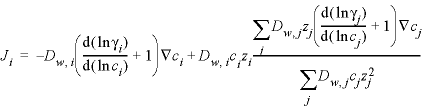
the diffusive flux is calculated by (see also Notes):
where i indicates the species; Ji
is the flux (mol m -2 s -1 , mole
per square meter per second); ![]() is the (temperature corrected) tracer diffusion coefficient (m 2 /s); ε is the water-filled (or
accessible) porosity (unitless); n is an empirical exponent, known
from Archie’s law to be about 1; γ i
is the activity-coefficient (unitless); ci is the concentration (mol/m
3 , mole per cubic meter); grad( ci ) is the concentration
gradient (mol/m 4 , mole per meter to the fourth power) , which
may be different in free (uncharged) pore water and in the Donnan pore space on
a surface (see Notes); and CBti is
the charge balance term (Appelo and Wersin, 2007, see the Notes). The
tracer diffusion coefficients are defined with keyword SOLUTION_SPECIES in
phreeqc.dat for 25 °C, and corrected to temperature T (K) of the
solution as follows:
is the (temperature corrected) tracer diffusion coefficient (m 2 /s); ε is the water-filled (or
accessible) porosity (unitless); n is an empirical exponent, known
from Archie’s law to be about 1; γ i
is the activity-coefficient (unitless); ci is the concentration (mol/m
3 , mole per cubic meter); grad( ci ) is the concentration
gradient (mol/m 4 , mole per meter to the fourth power) , which
may be different in free (uncharged) pore water and in the Donnan pore space on
a surface (see Notes); and CBti is
the charge balance term (Appelo and Wersin, 2007, see the Notes). The
tracer diffusion coefficients are defined with keyword SOLUTION_SPECIES in
phreeqc.dat for 25 °C, and corrected to temperature T (K) of the
solution as follows:
where η is the viscosity of water.
When -multi_D is false , the diffusive flux is calculated
with J i = - D p
× grad( c i ), where
D p is the same for all species (defined with identifier -diffusion_coefficient as in Line 9) and not corrected
for changes of temperature.
Note that PHREEQC assumes that, for diffusion, the cell contains
water exclusively, and uses the pore water diffusion coefficient for
calculating the flux. (The effective diffusion coefficient (D e ) is
for a volume of grains and pores together, and is related to D p
as follows: D e = D p ε ). The identifier -stagnant
allows for nonuniform porosities, nonuniform tortuosities,
and other variations in the diffusion domain, provided mixing factors among
cells are defined explicitly in the input file with MIX data blocks.
( True or False
)--If true , multicomponent diffusion is calculated; if false
, diffusion is calculated with the diffusion coefficient given in Line 9 .
default_Dw --The diffusion coefficient (m 2 /s at 25 °C) given to
solute species for which -dw is not
defined in keyword SOLUTION_SPECIES . T he
value must be used when calculating explicit mixing factors for stagnant cells.
Default is 0 m 2 /s.
porosity --The porosity filled with
free and Donnan pore water in the cells; the porosity is a fraction of
a representative volume of the porous medium (unitless). Initially all cells
are defined with the same porosity . The
porosity for a cell can be changed in any keyword data block that supports
Basic programming (RATES, USER_GRAPH, USER_PRINT, and USER_PUNCH) by using the PHREEQC
Basic function CHANGE_POR(porosity, cell_no). The
porosity in a cell can be retrieved with the function GET_POR(cell_no). Default is 0 (unitless).
porosity_limit --The porosity limit, below which diffusion stops. Default is 0
(unitless).
Archie_n --The exponent n used for calculating the pore-water diffusion
coefficient (D p, i ) from the tracer diffusion coefficient (D w, i ), Dp, i = Dw, i
ε n, where ε is the water filled (or the
accessible) porosity (unitless), and n is an empirical exponent that varies
from approximately 0.9 to 1.2 (Grathwohl, 1998; Van Loon and others, 2007) but
may be higher for diffusion perpendicular to the bedding plane. The parameter ![]() (approximately 1 / ε
wn) is the tortuosity factor, which accounts for the
longer diffusion path for a particle in a porous media than in pure water.
(approximately 1 / ε
wn) is the tortuosity factor, which accounts for the
longer diffusion path for a particle in a porous media than in pure water.
True or False—Optional argument to use ionic strength to correct the
diffusion coefficients for aqueous species (dw) in
electromigration calculations. Default is False.
Line 22: -interlayer_D ( True or False ) interlayer_porosity
interlayer_porosity_limit interlayer_tortuosity_factor
-interlayer_D --Enables or disables the calculation of interlayer diffusion in
swelling clay minerals. If -interlayer_D
is true , -multi_D also must be true , and
the -multi_D parameters must be set
as explained with Line 21. Optionally, interlayer_D
or -int [ erlayer_D ] (as with all
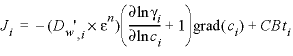
identifiers, case insensitive). The flux in the interlayers is calculated for
the cations associated with X- (as defined with keyword EXCHANGE):
Ji = - ![]() × mCEC ×
grad( βι ) + CBti,
× mCEC ×
grad( βι ) + CBti,
where, i indicates an aqueous species,
Ji is the flux (mol m -2 s -1 ), Dw',i is the temperature
corrected diffusion coefficient, ![]() is the interlayer tortuosity
factor (unitless), mCEC is the concentration of total
X-, mol(X-) / (m3 interlayer water), where (m3 interlayer water) = (m3 free
pore water + m3 Donnan water) × ( εIL
/ ε ), grad( βι ) is the gradient of the
equivalent fraction of species i on the exchange
sites (1/m), and CBti is the charge balance term
(Appelo and Wersin, 2007). The tracer diffusion coefficients are defined with
keyword SOLUTION_SPECIES in phreeqc.dat for 25 °C and are
corrected to temperature T (K) of the solution with the equation Dw' = (Dw )298 ×
is the interlayer tortuosity
factor (unitless), mCEC is the concentration of total
X-, mol(X-) / (m3 interlayer water), where (m3 interlayer water) = (m3 free
pore water + m3 Donnan water) × ( εIL
/ ε ), grad( βι ) is the gradient of the
equivalent fraction of species i on the exchange
sites (1/m), and CBti is the charge balance term
(Appelo and Wersin, 2007). The tracer diffusion coefficients are defined with
keyword SOLUTION_SPECIES in phreeqc.dat for 25 °C and are
corrected to temperature T (K) of the solution with the equation Dw' = (Dw )298 × ![]() ×
× ![]() , where η is
the viscosity of water.
, where η is
the viscosity of water.
( True or False
)--If true , interlayer diffusion is calculated; if false
, interlayer diffusion is not calculated .
interlayer_porosity --The porosity of interlayer water, a fraction of the total volume . Default is 0 (unitless) .
interlayer_porosity_limit --The porosity of interlayer water, below which interlayer
diffusion stops. Default is 0 (unitless).
interlayer_tortuosity_factor --The tortuosity factor for interlayer diffusion, ![]() (unitless). Default is 100.0.
(unitless). Default is 100.0.
Line 23: -porosities list of porosities
-porosities--Defines porosity of each cell for diffusive
transport simulations (m). Optionally, po[rosities]
or -po[rosity].
list of porosities--Porosity of each cell (unitless). Any number
of porosities up to the total number of cells (cells) may be entered. If cells is greater than the number of lengths entered, the final
value read will be used for the remaining cells. Multiple lines may be used.
Repeat factors can be used to input multiple data with the same value; in the
Example data block, 4*0.30 is interpreted as 4 values of 0.30. The values
entered here take pecedence ofver
the value given with -multi_D. If one stangant layer is defined together with an exchange-factor
> 0 (‘-stagnant 1 4e-6 0.3 0.1’), the mobile (here = 0.3) and immobile (here
= 0.1) porosities defined with -stagnant are used. If -interlayer_d
is defined, then the total porosity for a cell is the sum of the porosity
defined here and the porosity defined by -interlayer_d.
-fix_current--Current in a column
experiment. Default is 0 at startup. Optionally, fix_current,
-fi[x_current], or current, or -cu[rrent].
current--Electrical current, Default is 0 amperes.
Line 25: -implicit (True or False) max_mix_factor
[min_LM]
-implicit--Select implicit algorithm that allows for for large time steps when multicomponent diffusion is
calculated. Optionally, implicit or -im[plicit].
(True or False)--True, implicit method
or false, explicit method is used for multicomponent diffusion calculations.
max_mix_factor--Maximum mix factor allowed, where max_mix_factor
= D * Δt / Δx2. The default value of max_mix_factor = 1, but it can be increased often to >
4, depending on the required accuracy and the chemistry of the system, and the
calculations will be about an order of magnitude faster.With implicit true, electro-migration
calculation is more stable and usually avoids the (possibly) disturbing
warnings of ‘negative moles’. The implicit calculations have been implemented
for a regular column and, optionally a single stagnant cell. The implicit
method is not implemented for interlayer diffusion.
min_LM--Defines a minimum log10 molality for including a species in
multicomponent diffusion calculations. If log10 concentration of an aqueous
species is less than this value in all cells, then the species is not included
in the multicomponent diffusion calculation. Default is -30; a value of -12 is
reasonable.
Line 26: -same_model cell ranges
-same_model--Use the chemical model
structure of the previous calculation for specific cells Optionally, same_model or -sa[me_model].
cell ranges--One or more ranges of cell numbers, where a range
is either a single cell number or the beginning and ending cell number
separated by a hyphen. The composition of the cells in a range are set to the
values of the preceding cell number. For example, -same_model
2-5 8-11 use for cells 2-5 the model defined for cell 1, and for cells 8-11 the
model defined for cell 7.
Notes
The advective-dispersive transport capabilities of PHREEQC are
derived from a formulation of 1D, advective-dispersive transport presented by
Appelo and Postma (2005). The 1D column is defined by a series of cells (number
of cells is cells ), each of which has the
same pore volume. Lengths are defined for each cell and the time step ( time step ) gives the time necessary for
a pore volume of water to move through each cell. Thus, the velocity of water
in each cell is determined by the length of the cell divided by the time step.
In the Example data block, a column of five cells ( cells
) is modeled and 5 pore volumes of filling solution are moved through the
column ( shifts / cells is 5). The total time of the
simulation is 25 yr (year) (![]() ). The
total length of the column is 6 m (four 1-m cells and one 2-m cell).
). The
total length of the column is 6 m (four 1-m cells and one 2-m cell).
At each shift, advection is simulated by moving solution cells
- 1 to cell cells , solution cells -
2 to cell cells - 1, and so on, until solution 0 is moved to cell
1 (upwind scheme). With flux-type boundary conditions, the dispersion steps
follow the advective shift. With Dirichlet boundary conditions, the dispersion
step and the advective shift are alternated. After each advective shift and
dispersion step, kinetic reactions and chemical equilibria are calculated. The
moles of pure phases and the compositions of the exchange assemblage, surface
assemblage, gas phase, solid-solution assemblage, and kinetic reactants in each
cell are updated after each chemical calculation.
For advective transport, the influent solution must be defined,
otherwise the program stops with an error message. Solution 0 is the influent
with -flow_direction forward ; solution cells + 1 is the
influent when the flow is backward . If the effluent (solution
cells + 1, for direction forward ) is
not defined, the program copies it from the effluent boundary cell in the
column. A closed boundary condition is not possible with advective flow, and
the boundary condition will be changed to a flux boundary condition. Likewise,
a flux-boundary condition is not possible when pure diffusion is modeled, and
the boundary condition will be changed to a closed boundary condition.
The -time_step
identifier defines the length of time associated with each advective shift or
diffusion period. The program may subdivide this time step into smaller
dispersion time steps if necessary to calculate dispersion accurately. Each
dispersion time step may be further subdivided to integrate the kinetic
reactions (KINETICS data block).
Kinetic reactions are likely to slow the calculations by a factor of six or
more compared to pure equilibrium calculations.
The numerical scheme is for cell-centered concentrations, which
has consequences for data interpretation. Thus, the composition in a boundary
cell is a half-cell distance away from the column outlet and needs a half time
step to arrive at (or from) the column end. The half time step must be added to
the total residence time in the column when effluent from a column is simulated
[use (TOTAL_TIME + time step / 2) for time, see See 1D
Transport: Kinetic Biodegradation, Cell Growth, and Sorption, or ((STEP_NO
+ 0.5) / cells ) for pore volumes, see See Transport
and Cation Exchange]. The kinetics time for advective transport into the
boundary cell is the advective time step divided by 2. Also, the cell-centered
scheme does not account for dispersion in the border half-cell in case of a
flux boundary condition. The identifier -correct_disp
provides an option to correct the ignored dispersion by increasing the dispersivity for all cells in the column by the appropriate
amount. The correction will improve the comparison with analytical solutions
for conservative elements when the number of cells is small.
A “dual porosity” model, in which part of the porosity allows
advective flow and part of the porosity is accessible only by diffusion, can be
developed with a first-order exchange model or with finite differences, and
both approaches can be defined in terms of a mixing among cells (see “Transport
in Dual Porosity Media” in Parkhurst and Appelo, 1999). With the TRANSPORT
data block, one column of mobile cells is used to represent the part of the
flow system in which advection occurs, and then additional immobile cells
connected to the mobile cells are used to represent the stagnant zone that is
accessible only by diffusion. The stagnant zone can be defined to be parallel
or perpendicular to the column of mobile cells or to be a combination of the
two by proper definition of mixing factors in MIX data blocks. A shortcut is
available for the classical formulation of a dual porosity medium with a
first-order rate of exchange. In this case, -stagnant is used
to define one stagnant cell for each mobile cell ( stagnant_cells
= 1), an exchange factor ( exchange_factor )
for the exchange between immobile and mobile cells, and the porosities ![]() and
and ![]() for the mobile and immobile
cells.
for the mobile and immobile
cells.
Thermal diffusion can be modeled for a stagnant zone with
first-order exchange between mobile and immobile cells. Thermal exchange is
calculated after subtracting the part of the exchange that is associated with
hydrodynamic diffusion (see “Transport of Heat” in Parkhurst and Appelo, 1999).
PHREEQC uses the value of the diffusion coefficient to find the
correct heat exchange factor, and the value entered with identifier -diffusion_coefficient should be the same as has
been used to calculate the exchange factor ![]() (see equation 125 in Parkhurst and Appelo, 1999).
(see equation 125 in Parkhurst and Appelo, 1999).
Most of the information for advective-dispersive transport
calculations must be entered with other keyword data blocks.
Advective-dispersive transport assumes that solutions with numbers 1 through cells
have been defined by using SOLUTION,
SOLUTION_SPREAD, or SAVE data blocks. In addition the infilling solution must be defined. If -flow_direction is forward
, solution 0 is the infilling solution; if -flow_direction
is backward , solution cells + 1 is the
infilling solution, if -flow_direction
is diffusion_only , then infilling
solutions at both column ends are optional. If stagnant zones are modeled,
solution compositions for the stagnant-zone cells must be defined with SOLUTION, SOLUTION_SPREAD, or SAVE data blocks.
Pure-phase assemblages may be defined with EQUILIBRIUM_PHASES or SAVE, with the number of the
assemblage corresponding to the cell number. Likewise, an exchange assemblage,
a surface assemblage, a gas phase, or a solid-solution assemblage can be
defined for each cell through EXCHANGE,
SURFACE, GAS_PHASE, SOLID_SOLUTIONS, or SAVE keywords, with the identifying
number corresponding to the cell number. Kinetically controlled reactions can
be defined for each cell through the KINETICS
data block. Note that ranges of numbers can be used to define multiple
solutions, exchange assemblages, surface assemblages, gas phases,
solid-solution assemblages, or kinetic reactions simultaneously and that SAVE allows definition of a range of
numbers. Constant-rate reactions can be defined for mobile or immobile cells
through REACTION data blocks,
again with the identifying number of the REACTION data block corresponding to
the cell number. REACTION_TEMPERATURE
data blocks can be used to specify the initial temperatures of the cells in the
transport simulation. Temperatures in the cells may change during the transport
simulation depending on the temperature distribution and the temperature
retardation factor defined by -thermal_diffusion . REACTION_PRESSURE data blocks can be
used to set the pressure in each cell.
By default, the composition of the solution, pure-phase
assemblage, exchange assemblage, surface assemblage, gas phase, solid-solution
assemblage, and kinetic reactants are printed for each cell for each shift. Use
of -print_cells and -print_frequency will limit the amount of data
written to the output file. If -print_cells has been defined then only the specified cells will be
written; otherwise, all cells will be written. The identifier -print_frequency will restrict writing to the
output file to those shifts that are evenly divisible by print_modulus . In the
Example data block, results for cells 1, 2, 3, and 5 are written to the output
file after each integer pore volume (5 shifts) has passed through the column.
Data written to the output file can be further limited with the keyword PRINT (see -reset false ).
If a SELECTED_OUTPUT
data block has been defined, then selected data are written to the
selected-output file. Use of -punch_cells and
-punch_frequency in the TRANSPORT
data block will limit the data that are written to the selected-output file. If
-punch_cells has
been defined then only the specified cells will be written; otherwise, all
cells will be written. The identifier -punch_frequency
will restrict writing to the selected-output file to those shifts that
are evenly divisible by punch_modulus . In the Example data block, results are written to the
selected-output file for cells 2, 3, 4, and 5 after each integer pore volume (5
shifts) has passed through the column.
At the end of an advective-dispersive transport simulation, all
the physical and chemical data (for example, compositions of solutions,
equilibrium-phase assemblages, surfaces, exchangers, solid solutions, and
kinetic reactants) are automatically saved and are identified by the cell
number in which they reside. These data are available for subsequent
simulations within a single run. Transient conditions can be simulated by
including subsequent SOLUTION and TRANSPORT
data blocks, which may define new chemical boundary and transport conditions.
Only parameters that differ from the previous advective-dispersive transport
simulation need to be redefined, such as new infilling solution (SOLUTION 0), a change from advection
to diffusion only ( -flow_direction diffusion_only ), or a change in flow direction
from forward to backward ( -flow_direction
backward ). All parameters not specified in the new TRANSPORT
data block remain the same as the previous advective-dispersive transport
simulation. Normally, the diffusion coefficient, lengths of cells, dispersivities, and stagnant zone definitions remain the
same through all advective-dispersive transport simulations and thus need not
be redefined.
For long advective-dispersive transport calculations, it may be
desirable to save intermediate states in the calculation, either because of
hardware failure or because of nonconvergence of the numerical method. The -dump_frequency identifier allows intermediate
states to be saved at intervals during the calculation. The -dump identifier
allows the definition of a file name in which to write these intermediate
states. The dump file is formatted as an input file for PHREEQC, so
calculations can be resumed from the point at which the dump file was made. The
-dump_restart identifier allows a
shift number to be specified from which to restart the calculations.
With the identifiers -multi_D
and -interlayer_D , diffusion can be calculated as a multicomponent process
in uncharged (“free”) pore water, in electrostatic double layer (EDL, referred
to as the Donnan pore space) water at charged surfaces, and in interlayer water
of swelling clay minerals. Each solute species or surface defined with -dw greater than zero diffuses at its own speed,
while overall, charge balance is maintained (Vinograd and McBain, 1941; Appelo
and Wersin, 2007). Instead of concentration, as in Fick’s laws, the
thermodynamic potential forms the basis for calculating the multicomponent
flux:
μi = μi0 + RT ln ai + ziFψ,
(9)
where μi0 is the standard thermodynamic potential of species i (J/mol, joule per mole), R is the gas constant (8.314 J
K-1mol-1), T is the absolute temperature (K), ai is the activity (unitless), zi
is charge number (unitless), F is the Faraday constant (96485 J V-1eq-1), and
ψ is the electrical potential (V). The activity is related to
concentration ci (here, mol/m3) by ai = γi
ci/c0, where γi is the activity coefficient
(unitless) and c0 is the standard state (here 1.0 mol/m3). The diffusive flux
of i as a result of chemical
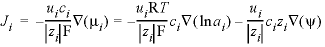
and electrical potential gradients is
 , (10)
where Ji is the flux of species i (mol
m-2s-1), ui is the mobility (m2 s-1V-1, square meter
per second per volt), ci is the concentration (mol/m3), zi is charge number
(unitless), ![]() is the gradient of the chemical potential (J mol-1m-1, joule per
mole per meter), and similarly for the gradients of lnai
and ψ. If the electrical current is zero,
is the gradient of the chemical potential (J mol-1m-1, joule per
mole per meter), and similarly for the gradients of lnai
and ψ. If the electrical current is zero,  , equation 10 can be
rearranged to solve for the gradient of the electrical potential:
, equation 10 can be
rearranged to solve for the gradient of the electrical potential:
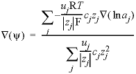 , (11)
where the variables are linked with species j to indicate their
origin from the zero-charge transfer condition. With ai = γi
ci/c0 and cid(lnci) =
d(ci), the gradient of the activity becomes:
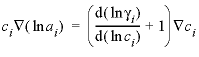
 , (13)
equation 10 can be
recast completely in known model variables:
 .
(14)
.
(14)
The diffusion coefficients are given in the database phreeqc.dat
for 25oC with identifier -dw, and
corrected to temperature TK (Kelvin) of the solution with
(Dw)TK
= (Dw)298 × (TK / 298) × (viscos_0, 298 / viscos_0,
TK),
where viscos_0 is the
viscosity of pure water at the indicated temperature. For calculating
electro-migration, Dw can be corrected for ionic
strength like in PHREEQC's SC calculation if the sixth argument of -multi_D is set to true.
Dw can be corrected for viscosity by defining
the exponent a_v_dif, the 7th parameter in -dw, in SOLUTION_SPECIES. Dw can
be changed in a USER_ keyword with setdiff_c("name", Dw, a_v_diff). For example,
setdiff_c("H+", 9.31e-9,
1).
Appelo and Wersin (2007) have
shown that the thermodynamic potential gradients are the same in free pore
water and in EDL water (the Donnan pore space); only the concentrations are
different in the two water types. The concentration in the Donnan pore space
is:
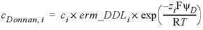 , (15)
where erm_DDLi is the enrichment factor
in the Donnan pore space, defined with identifier -erm_ddl
in keyword SOLUTION_SPECIES, and ψD is the potential in the Donnan pore space.
Accordingly, for calculating the flux through the Donnan space, if -only_counter_ions is false
, ci in equation 14 is
replaced by cDonnan, i for
the fraction of Donnan water in the pore space. If -only_counter_ions
is true , the concentration gradient in free pore water is
used for counter-ions (ci in equation
14 is not replaced for counter-ions), and for co-ions the flux is zero
(their concentration is zero), see below.
Diffusion of exchangeable cations can be calculated when they are
defined with exchange species X - , as in the databases phreeqc.dat and
wateq4f.dat. The concentration of an exchangeable species is
ci = γι × βι × CEC / zi, (16)
where ci is the concentration of species i
(mol/m3 interlayer water), γι is the
activity coefficient, defined with -gamma in keyword EXCHANGE_SPECIES, β is the
equivalent fraction of the exchangeable species, and CEC is the exchange
capacity (eq/m3, equivalent per cubic meter of interlayer water), defined as
moles X- in keyword EXCHANGE (the
volume of interlayer water is calculated from the interlayer porosity, as
explained below). For calculating the flux through the interlayer space, ![]() in equation 14 is replaced by
in equation 14 is replaced by ![]() .
.
The actual mass transfer is found by multiplying the flux by the
surface area, which PHREEQC calculates either from the amount of water in a
cell and the cell length in a regular column, or from the mixing factor defined
for stagnant cells, assuming a density of water of 1 kg/L. Thus, in a regular
column, the surface area for diffusion between two cells i
and j is
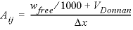 , (17)
where Aij is the surface area (m2), wfree
is kgw defined with -water in
keyword SOLUTION, VDonnan is the volume of water in the Donnan pore space,
equal to Asurf × tDonnan,
the product of the area of the surface (m2) and the thickness of the Donnan
layer (m), both defined in keyword SURFACE,
and Δx is the cell length (m) defined with -lengths
.
For stagnant cells, the mixing factor is multiplied by the ratio
of the diffusion coefficient of a species and the default diffusion coefficient
that is used when calculating the mixing factor. The mixing factor is given by
equation 128 of the PHREEQC version 2 manual (Parkhurst and Appelo, 1999) or
equation S2 of Appelo and Wersin, 2007):
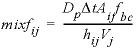 , (18)
where mixf ij
is the mixing factor between cells i and j, defined
with keyword MIX. D p
is the pore water diffusion coefficient, given by D p = D w
ε n ,
where D w is the default diffusion coefficient; ε is the
porosity; and n is Archie’s factor, all defined with identifier -multi_D . Δt is the
time step defined with -time_step . f bc is a correction
factor that equals 2 for constant concentration boundary cells and is 1
otherwise, hij is the distance between the midpoints
of cells i and j, and Vj is
the volume of pore water in cell j for which the mass transfer is calculated.
The mixfij that is defined in the input file must be
calculated with a volume Vj of 0.001 m3. PHREEQC will
adapt the value of mixfij by using the actual amount
of water in the cell, which is given by (w free /1000 + VDonnan). Furthermore, (according to equation 18) the mixing factor for
individual species is multiplied by D w, i
/D w .
For interlayer diffusion, PHREEQC calculates the surface area by
 , (19)
where εIL is the porosity occupied
by interlayer water, defined with identifier -interlayer_D , and ε is
the porosity of free and Donnan pore water together, defined with -multi_D . For stagnant cells, the mixing factor is
multiplied with the ratio of the interlayer porosity and the free and Donnan
porosity, and with the ratio of the diffusion coefficients, and of the inverse
tortuosity coefficients. If the surface areas and (or) the porosities are
different for the two cells, the harmonic mean is used (see See Modeling
Diffusion of HTO, 36Cl-, 22Na+, and Cs+ in a Radial Diffusion Cell, in Examples).
For the Donnan pore space, the enhanced concentration gradient for
counter-ions and the decreased concentration gradient for co-ions is applied if
identifier -only_counter_ions is false
in keyword SURFACE. If identifier -only_counter_ions is true
, the concentration of the co-ions is zero in the Donnan space, and also
the flux of the co-ions is zero. In this case, the concentration gradient of
counter-ions in free pore water is used for the Donnan pore space for two
reasons. First, because with only counter ions in the Donnan pore space, the
concentrations of the counter-ions will be smaller than in free pore water if
the surface charge is smaller than the charge of the co-ions in solution. This
could give unrealistic gradients when surface charges are different from cell
to cell. The second reason is that it allows direct comparison of
multicomponent results of PHREEQC with traditional calculations in which Fick’s
laws are used to model the behavior of individual tracers in clays and
clay-containing rocks.
Example problems
The keyword TRANSPORT is used in example problems
11, 12, 13, 15, and 21. Examples of multicomponent
diffusion are given in Appelo and Wersin (2007), supplementary information,
Appelo and others (2008) and (2010), and in
http://www.hydrochemistry.eu/exmpls/index.html#new (accessed June 25, 2012). An
example of interlayer diffusion is available in
http://www.hydrochemistry.eu/exmpls/opa_col.html#new2 (accessed June 25, 2012).
Related keywords
ADVECTION, EQUILIBRIUM_PHASES, EXCHANGE, GAS_PHASE, KINETICS, MIX, PRINT, REACTION, REACTION_TEMPERATURE, SAVE, SELECTED_OUTPUT, SOLID_SOLUTIONS, SOLUTION, and SURFACE.