| Next || Previous || Top |
Example 12--Advective and Diffusive Flux of Heat and Solutes
The following example demonstrates the capability of PHREEQC to calculate transient transport of heat and solutes in a column or along a 1D flowline. A column is initially filled with a dilute KCl solution at 25 °C in equilibrium with a cation exchanger. A KNO
3
solution then advects into the column and establishes a new temperature of 0 °C. Subsequently, a sodium chloride solution at 24 °C is allowed to diffuse from both ends of the column, assuming no heat is lost through the column walls. At one end, a constant boundary condition is imposed, and at the other end, the final cell is filled with the sodium chloride solution and a closed boundary condition is prescribed. For the column end with a constant boundary condition, an analytical solution is compared with PHREEQC results, for unretarded Cl
-
(R
= 1.0) and retarded Na
+
and temperature (
R
= 3.0). Finally, the second-order accuracy of the numerical method is verified by increasing the number of cells by a factor of three and demonstrating a decrease in the error of the numerical solution by approximately one order of magnitude relative to the analytical solution.
The input file for example 12 is shown in table 31. The EXCHANGE_SPECIES data block is used (1) to make the exchange constant for KX equal to NaX (log_k = 0.0), (2) to effectively remove the possibility of hydrogen ion exchange, and (3) to set activity coefficients for exchange species equal to their aqueous counterparts (
-gamma
identifier), so that the exchange between Na
+
and K
+
is linear and the retardation is constant. The influent, SOLUTION 0, is defined with temperature 0 °C and 24 mmol/kgw KNO
3
. All solutions are defined to be in equilibrium with atmospheric oxygen partial pressure. The column is discretized in 60 cells, which are filled initially with a 1-μmol/kgw KCl solution (SOLUTION 1-60). Each cell has 48 mmol of exchange sites, which are defined to contain only potassium by the data block EXCHANGE 1-60.
Table 31. Input file for example 12.
TITLE Example 12.--Advective and diffusive transport of heat and solutes.
|
Two different boundary conditions at column ends.
|
After diffusion temperature should equal Na-conc in mmol/l.
|
SOLUTION 0 24.0 mM KNO3
|
units mol/kgw
|
temp 0 # Incoming solution 0C
|
pH 7.0
|
pe 12.0 O2(g) -0.67
|
K 24.e-3
|
N(5) 24.e-3
|
SOLUTION 1-60 0.001 mM KCl
|
units mol/kgw
|
temp 25 # Column is at 25C
|
pH 7.0
|
pe 12.0 O2(g) -0.67
|
K 1e-6
|
Cl 1e-6
|
EXCHANGE_SPECIES
|
Na+ + X- = NaX
|
log_k 0.0
|
-gamma 4.0 0.075
|
|
H+ + X- = HX
|
log_k -99.
|
-gamma 9.0 0.0
|
|
K+ + X- = KX
|
log_k 0.0
|
gamma 3.5 0.015
|
EXCHANGE 1-60
|
KX 0.048
|
PRINT
|
-reset false
|
-selected_output false
|
-status false
|
SELECTED_OUTPUT
|
-file ex12.sel
|
-reset false
|
-dist true
|
-high_precision true
|
-temp true
|
USER_PUNCH
|
-head Na_mmol K_mmol Cl_mmol
|
10 PUNCH TOT("Na")*1000, TOT("K")*1000, TOT("Cl")*1000
|
TRANSPORT # Make column temperature 0C, displace Cl
|
-cells 60
|
-shifts 60
|
-flow_direction forward
|
-boundary_conditions flux flux
|
-lengths 0.333333
|
-dispersivities 0.0 # No dispersion
|
-diffusion_coefficient 0.0 # No diffusion
|
-thermal_diffusion 1.0 # No retardation for heat
|
END
|
|
SOLUTION 0 Fixed temp 24C, and NaCl conc (first type boundary cond) at inlet
|
units mol/kgw
|
temp 24
|
pH 7.0
|
pe 12.0 O2(g) -0.67
|
Na 24.e-3
|
Cl 24.e-3
|
SOLUTION 58-60 Same as soln 0 in cell 20 at closed column end (second type boundary cond)
|
units mol/kgw
|
temp 24
|
pH 7.0
|
pe 12.0 O2(g) -0.67
|
Na 24.e-3
|
Cl 24.e-3
|
|
EXCHANGE 58-60
|
NaX 0.048
|
PRINT
|
-selected_output true
|
TRANSPORT # Diffuse 24C, NaCl solution from column end
|
-shifts 1
|
-flow_direction diffusion
|
-boundary_conditions constant closed
|
-thermal_diffusion 3.0 # heat is retarded equal to Na
|
-diffusion_coefficient 0.3e-9 # m^2/s
|
-time_step 1.0e+10 # 317 years give 19 mixes
|
|
USER_GRAPH 1 Example 12
|
-headings Na Cl Temp Analytical
|
-chart_title "Diffusion of Solutes and Heat"
|
-axis_titles "Distance, in meters" "Millimoles per kilogram water", "Degrees celsius"
|
-axis_scale x_axis 0 20
|
-axis_scale y_axis 0 25
|
-axis_scale sy_axis 0 25
|
-initial_solutions false
|
-plot_concentration_vs x
|
-start
|
10 x = DIST
|
20 PLOT_XY x, TOT("Na")*1000, symbol = Plus
|
30 PLOT_XY x, TOT("Cl")*1000, symbol = Plus
|
40 PLOT_XY x, TC, symbol = XCross, color = Magenta, symbol_size = 8, y-axis 2
|
50 if (x > 10 OR SIM_TIME <= 0) THEN END
|
60 DATA 0.254829592, -0.284496736, 1.421413741, -1.453152027, 1.061405429, 0.3275911
|
70 READ a1, a2, a3, a4, a5, a6
|
# Calculate and plot Cl analytical...
|
80 z = x / (2 * SQRT(3e-10 * SIM_TIME / 1.0))
|
90 GOSUB 2000
|
100 PLOT_XY x, 24 * erfc, color = Blue, symbol = Circle, symbol_size = 10,\
|
line_width = 0
|
# Calculate and plot 3 times retarded Na and temperature analytical...
|
110 z = z * SQRT(3.0)
|
120 GOSUB 2000
|
130 PLOT_XY x, 24 * erfc, color = Blue, symbol = Circle, symbol_size = 10,\
|
line_width = 0
|
140 END
|
2000 REM calculate erfc...
|
2050 b = 1 / (1 + a6 * z)
|
2060 erfc = b * (a1 + b * (a2 + b * (a3 + b * (a4 + b * a5)))) * EXP(-(z * z))
|
2080 RETURN
|
-end
|
END
|
The TRANSPORT data block defines cell lengths of 1 m (
-lengths
1), no dispersion (
-dispersivities
0), no diffusion (
-diffusion_coefficient
0), and no retardation for temperature (
-thermal_diffusion
1). SOLUTION 0 is shifted 60 times into the column (
-shifts
60,
-flow_direction
forward), and arrives in cell 60 at the last shift of the advective-dispersive transport simulation. The boundary conditions at the column ends are of flux type (
-boundary_conditions
flux flux). In this initial advective-dispersive transport simulation, no exchange occurs because the exchange sites are already completely filled with potassium, and the concentrations and temperatures in the 60 cells evolve to 24 mmol/kgw KNO
3
and 0 °C. This result could be more easily achieved with SOLUTION data blocks directly, but the simulation demonstrates how transient boundary and flow conditions can be represented. The dissolved and solid compositions and the temperature of each cell of the column is automatically saved after each shift in the advective-dispersive transport simulation. The keyword PRINT is used to exclude all printing to the output file (
-reset
false).
In the next advective-dispersive transport simulation, diffusion is calculated from the column ends. The column composition and temperatures are initially the conditions produced by the first advective-dispersive transport calculation, except that an NaCl solution is now defined as solution 0, which diffuses into the top of the column, and as solution 60, which diffuses from the bottom of the column. The new SOLUTION 0 is defined with a temperature of 24 °C and with 24 mmol/kgw NaCl. The last cell (SOLUTION 60) also is defined to have this solution composition and temperature. The exchanger in cell 60 is defined to be in equilibrium with the new solution composition in cell 60 (EXCHANGE 60).
The TRANSPORT data block defines one diffusive transport period (
-shifts
1;
-flow_direction
diffusion). The boundary condition at the first cell is constant concentration, and at the last cell the column is closed (
-boundary_conditions
constant closed). The effective diffusion coefficient (
-diffusion_coefficient
) is set to 0.3×10
-9
m
2
/s, and the time step (
-time_step
) is defined to be 1.0×10
10
s. Because only one diffusive time period is defined (
-shifts
1), the total time modeled is equal to the time step, 1.0×10
10
s. However, the time step will automatically be divided into a number of time substeps to satisfy stability criteria for the numerical method. The heat retardation factor is set to 3.0 (
-thermal_diffusion
3.0). For Na
+
the ratio of exchangeable concentration (maximum NaX is 48 mmol/kgw) to solute concentration (maximum Na
+
= 24 mmol/kgw) is 2.0 for all concentrations, and the retardation is therefore
R
= 1 +
d
NaX/
d
Na
+
= 3.0, which is numerically equal to the temperature retardation.
The SELECTED_OUTPUT data block specifies the name of the selected-output file to be
ex12.sel
. The identifier “
-high_precision
true” is used to obtain an increased number of digits in the printing, and the identifiers
-dist
and
-temp
specify that the distance and temperature of each cell will be printed to the file. The USER_PUNCH data block is used to print concentrations of sodium, potassium, and chloride to the selected-output file in units of mmol/kgw, and USER_GRAPH plots the data.
In the model, the temperature is calculated with the (linear) retardation formula; however, the Na
+
concentration is calculated by the cation-exchange reactions. Even though the Na
+
concentration and the temperature are calculated by different methods, the numerical values should be the same because the initial and the transient conditions are numerically equal and the retardation factors are the same. The temperature and the Na
+
concentration are equal to at least 6 digits in the PHREEQC selected-output file, which indicates that the algorithm for the chemical transport calculations is correct for the simplified chemistry considered in this example. A further check on the accuracy is obtained by comparing simulation results with an analytical solution. For an infinite column with
C
x
= 0 for
t
= 0, and diffusion from
x
= 0 with
C
x=0
=
C
0
for
t
> 0 the analytical solution is
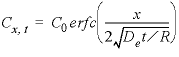 , (23)
where De is the effective diffusion coefficient and R is the retardation factor.
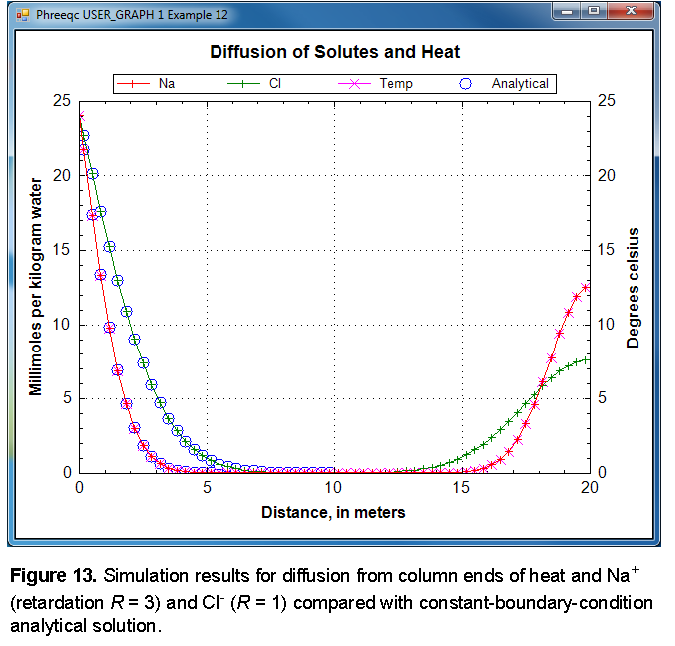
The PHREEQC results are compared with the analytical solution for Cl
-
and for temperature and Na
+
in figure 13 and show excellent agreement. Notice that diffusion of Cl
-
from the column ends has not yet “touched” in the mid-section, so that the column is still effectively infinite and the analytical solution is appropriate. Although both ends of the column started with the same temperature and concentration, at
x
= 0 m, the same temperature and concentrations are maintained because of the constant boundary condition. At
x
= 20 m (plotted at the midpoint of cell 60,
x
= 19.83 m), the temperature and concentrations decrease because of the closed boundary condition; no flux of heat or mass through this boundary is allowed, and the temperature and concentrations are diminishing because of diffusion into the column. The sodium concentration is not dissipating as rapidly as the chloride concentration because exchange sites must be filled with sodium along the diffusive reach.
Because this example has an analytical solution, it is possible to verify the second-order accuracy of the numerical algorithms used in PHREEQC. For a second-order method, decreasing the cell size by a factor of three should improve the results by about a factor of nine. The deviations from the analytical solution at the end of the time step are calculated at distances from 0.5 to 8.5 m in 0.5 m increments. The results are shown in table 32. As expected for a second-order method, the deviations from the analytical solution decreased by approximately an order of magnitude when the cell size was decreased by a factor of three.
Table 32. Numerical errors relative to the analytical solution for example 12 for a 20-cell and a 60-cell model.
|
Distance
|
Error in Cl concentration
|
|
Error in Na concentration
|
|
20-cell model
|
60-cell model
|
|
20-cell model
|
60-Cell model
|
|
|
|
|
|
|
|
|
|
|
|
|
|
|
|
|
|
|
|
|
|
|
|
|
|
|
|
|
|
|
|
|
|
|
|
|
|
|
|
|
|
|
|
|
|
|
|
|
|
|
|
|
|
|
|
|
|
|
|
|
|
|
|
| Next || Previous || Top |