 ,
,The following example simulates the chemical composition of the effluent from a column containing a cation exchanger (Appelo and Postma, 2005). Initially, the column contains a sodium-potassium-nitrate solution in equilibrium with the exchanger. The column is flushed with three pore volumes of calcium chloride solution. Calcium, potassium, and sodium react to equilibrium with the exchanger at all times. The problem is run two ways--by using the ADVECTION data block, which models only advection, and by using the TRANSPORT data block, which simulates advection and dispersive mixing.
The input file is listed in table 30. It starts with defining SOLUTION 0, which is the influent at cell 1 of the column. The column has 40 cells, and 40 solutions must be defined and numbered 1 through 40. The definition of a solution for each cell is mandatory. In this example, all cells contain the same solution, but this is not required. Solutions can be defined differently for each cell and could be changed by reactions in the current or preceding simulations (by using the SAVE keyword).
The amount and composition of the exchanger in each of the 40 cells is defined by the EXCHANGE 1-40 data block in the second simulation. The EXCHANGE data block could have been written in the first simulation where the initial solutions are defined, but generally, it is preferable to define additional reactants in separate simulations. The intervening END (between the first and second simulation) avoids a redundant reaction calculation in which the first solution defined (here SOLUTION 0) is reacted with the first exchanger that is defined (cell 1). The definition of an exchanger for cells in the column is optional. The number of the exchanger corresponds to the number of the cell in a column, and, if an exchanger exists for a cell number, it is used automatically in the transport calculations for that cell. In this column, each cell has 1.1 mmol exchange sites that are initially in equilibrium with solution 1. Note that the initial exchange composition is calculated by an initial exchange calculation that does not affect the composition of solution 1. At the end of this simulation, cell 1 is copied to cell 101, which includes the data blocks SOLUTION 1 and EXCHANGE 1. By copying cell 101 back to cell 1-40 at the end of the advection simulation, the column is reinitialized for the next transport calculation.
The ADVECTION data block need only include the number of cells and the number of shifts for the simulation. The calculation accounts for the numbers of pore volumes that flow through the cells; cell lengths are not used. The identifiers -punch_cells and -punch_frequency specify that data will be written to the selected-output file for cell 40 at each shift. The identifiers -print_cells and -print_frequency indicate that data will be written to the output file for cell 40 at every 20 shifts.
The SELECTED_OUTPUT data block specifies that the shift (or advection step number) and the total dissolved concentrations of sodium, chloride, potassium, and calcium will be written to the file ex11adv.sel . Pore volumes can be calculated from the shift number; one shift moves a solution to the next cell, and the last solution out of the column. PHREEQC calculates cell-centered concentrations, so that the concentrations in the last cell arrive one-half shift later at the column end. In this example, one shift represents 1/40 of the column pore volume. The number of pore volumes ( PV ) that have been flushed from the column is therefore PV = (number of shifts + 0.5) / 40. The number of pore volumes is calculated and printed to the selected-output file using the USER_PUNCH data block. Similarly, USER_GRAPH defines the chart with the same data plotted on-screen.
At the end of the advection calculation (ADVECTION), the initial conditions are reset for the advection and dispersion calculation (TRANSPORT) by copying solution and exchange 101 back to solution and exchange 1-40. SOLUTION 0 is unchanged by the ADVECTION simulation and need not be redefined. The TRANSPORT data block includes a much more explicit description of the transport process than the ADVECTION data block. The length of each cell ( -lengths ), the boundary conditions at the column ends ( -boundary_conditions ), the direction of flow ( -flow_direction ), the dispersivity ( -dispersivities ), and the diffusion coefficient ( -diffusion_coefficient ) can all be specified. The identifier -correct_disp should be set to true when modeling outflow from a column with flux boundary conditions. The identifiers -punch_cells , -punch_frequency , -print , and -print_frequency serve the same function as in the ADVECTION data block. The second SELECTED_OUTPUT data block specifies that the transport step (shift) number and total dissolved concentrations of sodium, chloride, potassium, and calcium will be written to the file ex11trn.sel . The USER_PUNCH data block from the advection simulation is still in effect and the pore volume at each transport step is calculated and written to the selected-output file. USER_GRAPH 1 is detached, which prevents adding any more data points. USER_GRAPH 2 is defined to make the curves distinct from the advection simulation [a plus (“+”) symbol is used for the calculated points] and to plot the analytical solution for chloride breakthrough with dispersion, which is
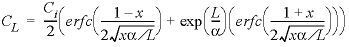
where C L is the concentration at the column-outlet (mol/kg H 2 O), C i is the concentration at the inlet (mol/kgw), x is the number of pore volumes (-), α is the dispersivity (m) and L is the length of the column (m).
The results for See Transport and Cation Exchange using the ADVECTION and TRANSPORT keywords are shown in figure 12. The concentrations in cell 40, which is the end cell, are plotted against pore volumes. The main features of the calculations are the same between the two transport simulations. Chloride is a conservative solute and arrives in the effluent after one pore volume. The sodium initially present in the column exchanges with the incoming calcium and is eluted as long as the exchanger contains sodium. The midpoint of the breakthrough curve for sodium occurs at about 1.5 pore volumes. Because potassium exchanges more strongly than sodium (because of the larger log K in the exchange reaction), potassium is released after sodium. Finally, when all of the potassium has been released, the concentration of calcium increases to the steady-state concentration in the influent.
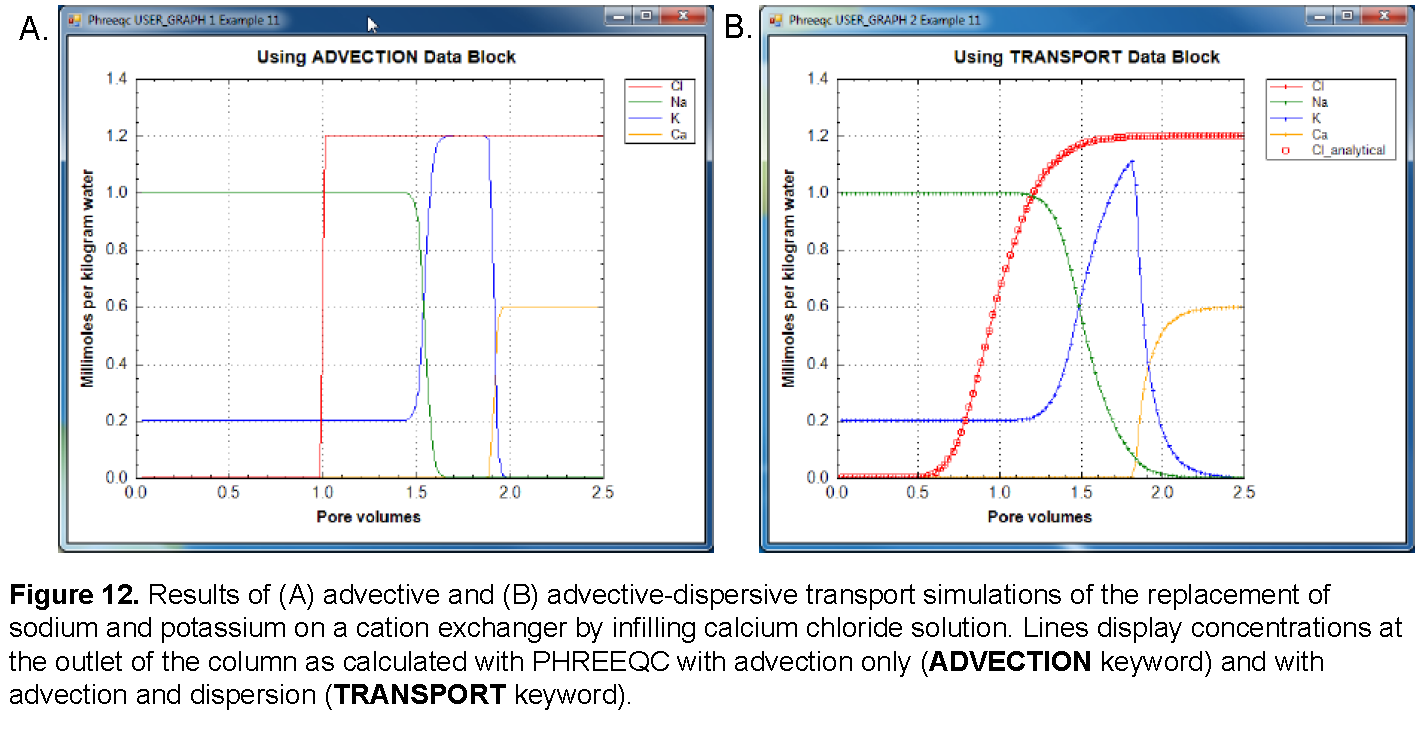
The concentration changes of sodium and potassium in the effluent form a chromatographic pattern, which often can be calculated by simple means (Appelo, 1994b; Appelo and Postma, 2005). The number of pore volumes needed for the arrival of the sodium-decrease front can be calculated with the formula  , where
  ,
,  indicates the change in sorbed concentration (mol/kgw), and
  indicates the change in solute concentration over the front. The sodium concentration in the solution that initially fills the column is 1.0 mmol/kgw, and the initial sorbed concentration of sodium is 0.55; the concentration of sodium in the infilling solution is zero, which must eventually result in 0 sorbed sodium. Thus,
 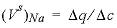 = (0.55 - 0)/(1 - 0) = 0.55 and
  , which indicates that the midpoint of the sodium front should arrive at the end of the column after 1.55 pore volumes.
Next, potassium is displaced from the exchanger. The concentration in solution increases to 1.2 mmol/kgw to balance the Cl
-
concentration, and then falls to 0 when the exchanger is exhausted. When potassium is the only cation in solution, it will also be the only cation on the exchanger. For potassium, 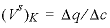 = (1.1 - 0)/(1.2 - 0) = 0.917 and
  pore volumes. It can be seen that the front locations for (
V
s
)
Na
and (
V
s
)
K
are closely matched by the midpoints of the concentration changes shown in figure 12.
pore volumes. It can be seen that the front locations for (
V
s
)
Na
and (
V
s
)
K
are closely matched by the midpoints of the concentration changes shown in figure 12.
The differences between the two simulations are due entirely to the inclusion of dispersion in the TRANSPORT calculation. The breakthrough curve for chloride in the TRANSPORT calculation coincides with an analytical solution to the advection dispersion equation for a conservative solute (Appelo and Postma, 2005), which is plotted in figure 12 with USER_GRAPH. The sum of the squared deviations for the first two pore volumes (transport step 80) is printed in the output file:
SSQD for Cl after 2 Pore Volumes: 7.985703292556e-005 (mmol/L)^2
The result shows that the calculations are in astonishingly good agreement. Without dispersion, the ADVECTION calculation produces a square-wave breakthrough curve for chloride. The characteristic smearing effects of dispersion are absent in the fronts calculated for the other elements as well, although some curvature exists because of the exchange reactions. The peak potassium concentration is larger in the ADVECTION calculation because dispersion is neglected.