This example demonstrates the capabilities of PHREEQC to calculate flow in a dual-porosity medium with diffusive exchange among the mobile and immobile pores. The flexible input format and the modular definition of additional solutions and reactants in PHREEQC allow inclusion of heterogeneities and various complexities within a 1D column. This example considers a column filled with small clay beads of 2 cm diameter, which act as dual porosity or stagnant zones. Both the first-order exchange approximation and finite differences are applied in this example, and transport of both a conservative and a retarded (by ion exchange) chemical is considered. It is furthermore shown how a heterogeneous column can be modeled by prescribing mixing factors to account for diffusion between mobile and immobile cells with the keyword MIX.
The first example input file, example 13A (table 33), is for a column with a uniform distribution of the stagnant porosity along the column. The 20 mobile cells are numbered 1 through 20. Each mobile cell, n , exchanges with one immobile cell, which is numbered 20 + 1 + n (cells 22 through 41 are immobile cells). All cells are given an identical initial solution and exchange complex, but these could be defined individually for each cell. It also is possible to distribute the immobile cells over the column non-uniformly, simply by omitting solutions for the stagnant cells that are not present. The connections between the mobile-zone and the stagnant-zone cells and among stagnant-zone cells can be varied along the column as well, but this requires that mixing factors among the mobile and immobile cells are prescribed by using the keyword MIX.
As defined in table 33, the column initially contains a 1 mmol/L KNO 3 solution in both the mobile and the stagnant zones (SOLUTION 1-41). An NaCl-NO 3 solution flows into the column (SOLUTION 0). An exchange complex with 1 mmol of sites is defined for each cell (EXCHANGE 1-41), and exchange coefficients are specified to give linear retardation R = 2 for Na+ (EXCHANGE_SPECIES). The first TRANSPORT data block is used to define the physical and flow characteristics of the first transport simulation. The column is 2 m in length and is discretized in 20 cells ( -cells ) of 0.1 m ( -lengths ). A pulse of five shifts ( -shifts ) of the infilling solution (SOLUTION 0) is introduced into the column. The length of time for each shift is 3,600 s ( -time_step ), which results in a velocity in the mobile pores vm = 0.1 / 3,600 = 2.78×10 -5 m/s. The dispersivity is set to 0.015 m for all cells ( -dispersivities ). The diffusion coefficient is set to 0.0 ( -diffusion_coefficient ).
The stagnant/mobile interchange is defined by using the first-order exchange approximation. The stagnant zone consists of spheres with radius r = 0.01 m, diffusion coefficient De = 3.×10 -10 m 2 /s, and shape factor fs ®1 = 0.21 (Parkhurst and Appelo, 1999, “Transport in Dual Porosity Media”, table 1). These variables give an exchange factor α = 6.8×10 -6 s -1 . Mobile porosity is εm = 0.3 ( -stagnant ) and immobile porosity εim = 0.1. For the first-order exchange approximation in PHREEQC, a single cell immobile zone and the parameters α, εm and εim are specified with -stagnant . This stagnant zone definition causes each cell in the mobile zone (numbered 1 through 20) to have an associated cell in the immobile zone (numbered 22 through 41). The PRINT data block is used to eliminate all printing to the output file.
Following the pulse of NaCl solution, 10 shifts of 1 mmol KNO 3 /L (second SOLUTION 0) are introduced into the column. The second TRANSPORT data block does not redefine any of the column or flow characteristics, but specifies that results for cells 1 through 20 ( -punch_cells ) be written to the selected output file after 10 shifts ( -punch_frequency ). The data blocks SELECTED_OUTPUT and USER_PUNCH specify the data to be written to the selected-output file, and USER_GRAPH plots the same data.
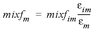
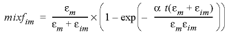
The mixing factors mixfm and mixfim for the first-order exchange approximation for this example are as follows (Parkhurst and Appelo, 1999, equations 121 and 123):
 . (25)
The retardation factors R m and R im do not appear in the formulas for mixf im and mixf m because in PHREEQC, the retardation is a consequence of chemical reactions. According to equations 24 and 25, for this example, the mixing factors are calculated to be mixfim = 0.20886 and mixfm = 0.06962. The mixing factors differ for the mobile cell and the immobile cell to account for the different volumes of mobile and immobile water.
In PHREEQC, a mixing of mobile and stagnant water is done after each diffusion/dispersion step. This means that the time step decreases when the cells are made smaller and when more diffusive steps (“mixruns”) are performed. A 20-cell model as in table 33 has one mixrun. A 100-cell model would have three mixruns, and the time step for calculating mixfim would be (3,600/5) / 3 = 240 s. A time step t = 240 s leads to mixfim = 0.01614 in the 100-cell model.
The input file with explicit mixing factors for a uniform distribution of the stagnant zones is given in table 34. The SOLUTION data blocks are identical to the previous input file (table 33). One stagnant layer without further information is defined (-stagnant 1, in the TRANSPORT data block). The mobile/immobile exchange is set by the mix fraction given in the MIX data blocks. The results of this input file are identical with the results from the previous input file in which the shortcut notation was used. However, the explicit definition of mix factors illustrates that a non-uniform distribution of the stagnant zones, or other physical properties of the stagnant zone, can be included in PHREEQC simulations by varying the mixing fractions that define the exchange among mobile and immobile cells.
 . (26)
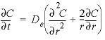
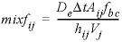
The calculation in finite differences can therefore be simplified to one (radial) dimension. The calculation follows the theory outlined in Parkhurst and Appelo (1999, section “Transport in Dual Porosity Media”). The stagnant zone is divided into a number of layers that mix by diffusion. In this example, the sphere is cut in five equidistant layers with Δ r = 0.002 m. Five stagnant layers are defined under keyword TRANSPORT with -stagnant 5 (table 35). Mixing is specified among adjacent cells in the stagnant layers with MIX data blocks; the mixing factors are calculated by See , and 28. For a neighbor cell, the mixing factor is
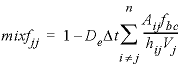 , (28)
where, D e is the effective diffusion coefficient, Δ t is the time interval, Vj is the volume of cell j (m3), Aij is the shared surface area of cell i and j (m2), hij is the distance between midpoints of cells i and j (m), and fbc is the correction factor for boundary cells (dimensionless). The values for mobile cell 1 and associated. immobile cells are given in table 36. The cells in the immobile layer are numbered as n + ( l × cells) + 1, where n is the number of a mobile cell, l is the number of the stagnant layer, and cells is the total number of mobile cells. In this example, the boundary cell in the stagnant zone for cell number 1 is cell number 22 and the other four stagnant layers are cell numbers 42, 62, 82, and 102, with number 102 being the innermost cell of the sphere, which is connected only to one other cell (cell 82). The volume of the mobile cell (cell 1) is expressed relative to the volume of a sphere of radius 0.01 m, by multiplying this volume by εm / εim (4.19×10 -6 × 0.3 / 0.1 = 1.26×10 -5 ). In table 36 the value for fbc is 1.72, as calculated with the following equation from Parkhurst and Appelo (1999, equation 127):
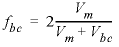 , (29)
where, V m is the volume of the mobile zone and V bc is the volume of the boundary cell that contacts the mobile zone. It is noted that using fbc = 1.81 slightly improves the fit to an analytical solution given in Crank (1975) for diffusion into spheres in a closed vessel (a beaker with solution and clay beads). However, changing fbc to 1.81 has little effect on the concentration profiles for the columns that are shown in figure 14, and various calculations have shown that fbc = 2 provides good results in general.
Note in table 35 that 121 solutions are defined, 1 through 20 for the mobile cells, and the rest for the immobile cells. The input file is identical with the previous one, except for -stagnant 5 and the mixing factors among the cells. Although not all the mixing factors are shown in table 35, the remaining mixing factors are identical for subsequent cells and their neighboring stagnant cells. In this example with clay beads, only radial (1D) diffusion is considered, and only mixing among cells in different layers is defined; however, it is possible to include mixing among the immobile cells of adjacent mobile cells.
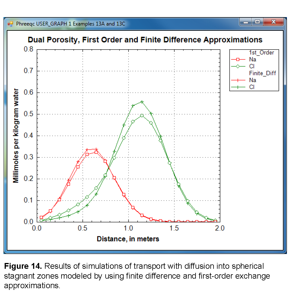
Figure 14 compares the concentration profiles in the mobile cells obtained with examples 13A and 13B with example 13C. The basic features of the two simulations are the same. The positions of the peaks, as calculated by the two simulations, are similar. The Cl - peak is near 1.2 m, but would be at about 1.45 m in the absence of stagnant zones. The integrated concentrations in the mobile porosity are about equal for the first-order exchange and the finite difference simulations. The exchange factor fs ®1 = 0.21 for the first-order exchange approximation appears to provide adequate accuracy for this simulation. However, the first-order exchange approximation produces lower peaks and more tailing than the more exact solution obtained with finite differences. Discrepancies can also appear as deviations in the breakthrough curve (Van Genuchten, 1985). The first-order exchange model is probably least accurate when applied to simulating the transport behavior of spheres; other shapes of the stagnant area can give a better correspondence. It is clear that the linear exchange model is much easier to apply because any explicit model requires the preparation of extended lists of mixing factors (notice that a separate simulation with USER_PUNCH can serve that purpose, as illustrated in examples 8 and 21), which change when the discretization is adjusted. The calculation time for a finite difference model with multiple immobile-zone layers also may be considerably longer than for the single immobile-zone layer of the first-order exchange approximation.
 (24)
(24) , (27)