This example illustrates how PHREEQC version 3 can simulate a diffusion experiment, as is now often performed for assessing the properties of a repository for nuclear waste in a clay formation. A sample is cut from a core of clay, enveloped in filters, and placed in a diffusion cell (see Van Loon and others, 2004, for details). Solutions with tracers are circulated at the surfaces of the filters, the tracers diffuse into and out of the clay, and the solutions are sampled and analyzed regularly in time. The concentration changes are interpreted with Fick’s diffusion equations to obtain transport parameters for modeling the rates of migration of elements away from a waste repository. Transport in clays is mainly diffusive because of the low hydraulic conductivity, and solutes are further retarded by sorption (cations) and by exclusion from part of the pore space (anions).
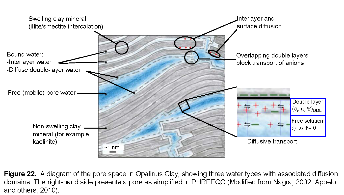
For calculating diffusion, one needs to account for the different diffusion coefficients of the tracers, the effect of the filters, and the properties of the clay. Figure 22 presents a schematic diagram of the processes in the clay (Appelo and others, 2010). The pores in the clay are lined with clay minerals that have a negative surface charge. The charge is partly neutralized by cations that are bound to the surface and partly by the electrostatic double layer that extends some distance into the pore. The double layer contains an excess of cations (counter-ions, in general) and a deficit of anions (co-ions, in general). In swelling clay minerals, such as montmorillonite, cations in the interlayer space also neutralize part of the negative charge. In comparison with concentration gradients that drive diffusion in free (uncharged) pore water, the gradient for a cation is magnified in the double layer, whereas the gradient for an anion is diminished, and the gradient for a neutral species remains the same. The charge in the double layer lowers the dielectric permittivity of the water, which enhances the ion-association of cations and anions into neutral species. Also, the viscosity of water may be higher than in free pore water. Where double layers overlap in pore constrictions, anions are impeded and forced to take longer paths, whereas cations and neutral species pass through unhindered.
PHREEQC has capabilities to model many of these diffusion processes. An averaged double layer composition can be calculated by using the identifier -Donnan in keyword SURFACE, which, in essence, neutralizes the surface charge. Solute species can be assigned an enrichment factor in the Donnan pore space to emulate the additional concentration change as a result of different ion association. For diffusion, the viscosity can be set differently with respect to free pore water. In this example, all these properties are adjusted for the tracers tritium (HTO), Na+, Cs+ and Cl- to simulate experimental results.
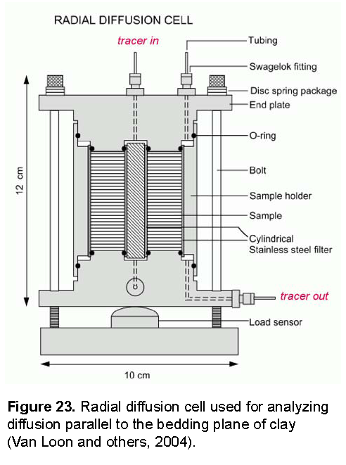
The experiments to be modeled were done in a radial diffusion cell, shown in figure 23. The radial cell enables measurement of diffusion parallel to the bedding plane of the clay (Van Loon and others, 2004). A solution with tracers is circulated at the surface of the inner filter, and another solution with the same major ions, but without tracers, contacts the surface of the outer filter. The latter solution is removed regularly and analyzed for the tracer that has diffused through the filters and the clay. Meanwhile, the outer solution is replaced by fresh solution, thus, maintaining tracer concentrations near zero in the outer solution. In the simulations, low solubility phases were defined to maintain small concentrations of tracers in the outer solution. The moles of precipitates of these phases give the accumulated mass that has diffused through the column.
For a linear column, PHREEQC calculates diffusion automatically by using the parameters entered with identifier -multi_D in keyword TRANSPORT. However, diffusion in the experiment is radial, and the filters have different properties than the clay. Also, the boundary solutions for the default (linear) column have a constant composition, whereas we want to know the concentration changes in these solutions during the diffusion experiment. All these experimental details can be simulated for a stagnant column by defining mixing factors among the individual cells with keyword MIX.
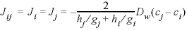
The mixing factors can be derived from Fick’s diffusion equations,  and
and  , which transform to finite differences for an arbitrarily shaped cell j:
 , (44)
where  is the concentration in cell
j
at the current time (mol/m3),
is the concentration in cell
j
at the current time (mol/m3),  is the concentration in cell
j
after the time step, Dw is the tracer diffusion coefficient (m2/s),
is the concentration in cell
j
after the time step, Dw is the tracer diffusion coefficient (m2/s),  is the time step (s), i is an adjacent cell,
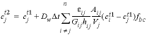
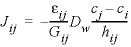
  is the porosity over the interface of cells i and j (unitless), Gij is the geometrical factor that corrects for tortuosity of the porous medium (unitless), hij is the distance between midpoints of the cells (m), Aij is the shared surface area of cells i and j (m2), Vj is the volume of cell j (m3), and fbc is a factor for boundary cells (unitless). The summation is for all cells (up to n) adjacent to j. When hij is equal for all cells, a central difference algorithm is obtained that has second-order accuracy [O(h)2] (Appelo and others, 2008). It is therefore advantageous to make the grid regular. However, the same accuracy is achievable for a heterogeneous domain, even with widely variable gridsize, if the harmonic mean of the parameters in
  is used. These parameters together, translate the tracer diffusion coefficient Dw into the effective diffusion coefficient De.
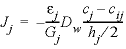
The harmonic mean can be derived in general (omitting the activity coefficient to simplify the formulas) as follows. The fluxes inside cells i and j and over the interface of the two cells must be the same and are given by:
 , (47)
where h is the cell length (m), and cij is the concentration at the interface. Substituting  = gi, in equation 46 and similarly in equation 47, the two equations can be combined while eliminating the concentration cij to give:
 . (48)
Multiplying the flux by the surface area, the time step, and the boundary factor, and dividing by the volume of the cell for which the concentration change is calculated (here, cell j), the mixing factor is obtained:
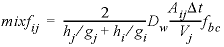 , (49)
where fbc is 2 for cells in contact with a constant concentration cell, and 1 otherwise. When calculating mixf, Vj is set to 10 -3 m 3 , and for Dw the default diffusion coefficient is used, entered with identifier -multi_D. In multicomponent-diffusion mode, PHREEQC adapts the volume Vj (entered as 10 -3 m 3 in equation 49), to the actual volume of water in cell j, and multiplies the mixing factor for each solute species a by the ratio of the tracer diffusion coefficient for a and the default diffusion coefficient (Dw, a / Dw).
To avoid numerical oscillations, it is necessary that mixf < 0.5, which can be realized by limiting the time step. This maximum permissible time step is usually determined by the cell with the smallest volume (in the model) and the fluxes of the proton, which normally has the highest tracer diffusion coefficient. However, if the proton concentration is sufficiently buffered by alkalinity or other species, and the solutions are uniform except for the tracers, the tracer with the highest Dw may be selected for calculating the maximum permissible time step. If, nevertheless, time steps are too large, PHREEQC warns that negative concentrations are calculated (and the program stops because the system reached an infeasible state), the time step can be subdivided. For example, -time_step 5e2 3 will subdivide the time step of 500 s in three equal ones of 166.7 s.
The input file in table 60 defines the physical and chemical properties of the clay pore space and writes the mixing factors for diffusional transport in the filters and the clay. The filters used by Van Loon have a geometrical factor of 4 for all the tracers, whether charged or not (Glaus and others, 2008). In the clay, the geometrical factor for HTO is 6.2. For cations, the geometrical factor appears to be 2 to 4 times smaller than for tritium. However, in this example (example 21), the same geometrical factor is used for both HTO and the cations; the smaller apparent geometrical factors are modeled by subdividing the pore space into free pore water and double-layer water. The concentrations of cations are higher in double-layer water than in free pore water, and hence, the concentration gradients of cations are also higher, which, as noted previously enhances their diffusion. In models that do not account for this physical aspect of the clay pore space, the faster diffusion is treated by diminishing the geometrical factor.
For anions, the geometrical factor is about 1.5 times larger than for tritium. This larger factor is related to narrowing of the pores, where overlapping double layers decrease the accessible porosity for anions and obstruct their passage (as noted above). The model accounts for the observed, smaller accessible porosity for anions relative to tritium and cations by the calculation of anion exclusion in the double layer.
The file starts with the tracer species, where, for the monovalent tracers 22Na+ (=“Na_tr+”) and Cs+, an enrichment factor for the double layer is entered with -erm_ddl in the SOLUTION_SPECIES data block. The enrichment is related to increased complexation of the polyvalent cations in the low dielectric permittivity of the double layer, and thus, more charge must be counterbalanced by monovalent cations. Sorption of Cs+ is much stronger than that of Na+, which is modeled by two surface complexes and one exchange reaction with large constants. The constants are based on the measured adsorption isotherm for Opalinus Clay, but may be generally applicable because they are associated primarily with strong sorption sites on illite. Next, the file writes SOLUTION 0-2 for a regular column, followed by SOLUTION 3,
which forms the start of the stagnant column and circulates at the inner filter of the diffusion cell. This solution contains the tracers and the amounts of water used in the experiment. The lines can be uncommented one by one to run the file successively with the different tracers and amounts of water. When SOLUTION 3 is calculated, USER_PUNCH is processed to write a SELECTED_OUTPUT file named radial, which contains the SOLUTION definitions for the cells in the filters and the clay, the mixing factors, and the TRANSPORT and USER_GRAPH data blocks. The Basic lines in USER_PUNCH do the following tasks:
The experiments with the tracers 22Na and Cs can be calculated together, because the tracer solutions contained identical amounts of water. Thus, when the 22Na profile has been plotted after 45 days, another TRANSPORT block is written to calculate diffusion of Cs during 1,000 days in total.
Following the END after USER_PUNCH, the file radial is loaded in the input file with INCLUDE$ and then processed. Before the file is included, writing to file radial is suspended (PRINT; -selected_output false), thus avoiding rewriting the file over and over again, each time a solution is calculated.
Three transport calculations with different tracers can be run with the input file (1) HTO, (2) 36Cl, and (3) 22Na and Cs together. To perform one of these three calculations, uncomment the appropriate line defining the tracer(s) in SOLUTION 3. Note that the length of the Cs experiment is about 1,000 days compared to less than 50 days for the other experiments; consequently, the Cs calculation is 20 times longer than the others.
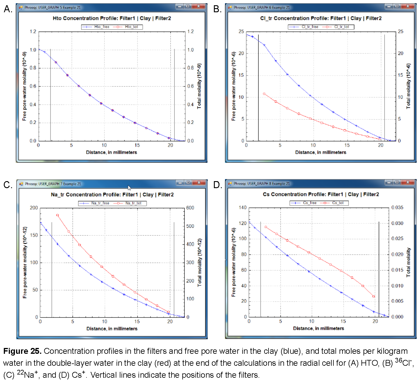
The results of the three calculations are shown in figures See Mass outflow (red) and corresponding flux (green) by diffusion through the radial cell for (A) HTO, (B) 36Cl-, (C) 22Na+, and (D) Cs+. Lines are modeled; symbols indicate measured data. and See Concentration profiles in the filters and free pore water in the clay (blue), and total moles per kilogram water in the double-layer water in the clay (red) at the end of the calculations in the radial cell for (A) HTO, (B) 36Cl-, (C) 22Na+, and (D) Cs+. Vertical lines indicate the positions of the filters.. As shown, the arrival times of the tracers that accumulate in the outer solution are delayed by the storage in pore water and the sorption on minerals in the clay. The delay increases in the order 36Cl- < HTO < 22Na+ < Cs+ (fig. 24). The total storage can be obtained from the graphs by extrapolating the straight-line segment of the accumulated mass to time zero (fig. 24) and reading the value from the secondary Y-axis (a negative number, because mass is lost). The flux, the derivative of the mass with time, shows that the accumulation of HTO, and of Cs+ in particular, decreases during the experiment (fig. 24) because the concentration is diminishing in the tracer solution. The volume of the solution with HTO, the first experiment performed, was relatively small (0.2 L) and insufficient to maintain a constant concentration for the inner solution. Sorption of Cs+ is so strong (more than 99.5 percent of Cs+ resides in the solid phase) that 1 L of inner solution simply contains insufficient mass to fill all the sorption sites on the clay. Figure 25 shows on the primary Y axis the concentration profile at the end of the diffusion periods, including concentrations in the inner filter, the free pore water of the clay, and the outer filter. The figure shows on the secondary Y axis the total moles, which includes moles sorbed and moles dissolved in free and double layer water, expressed per kilogram of total water. The two concentrations are the same for HTO (the concentration of HTO is the same in free and in double layer water), the free pore-water concentration of Cl- is twice the total concentration (the concentration of Cl- in the double layer is smaller than in free pore water), and the free pore-water concentrations of Na+, and particularly of Cs+, are smaller than the total concentrations because the cations have a higher concentration in the double layer than in free pore water, and because cations are sorbed on the surface and exchange sites.
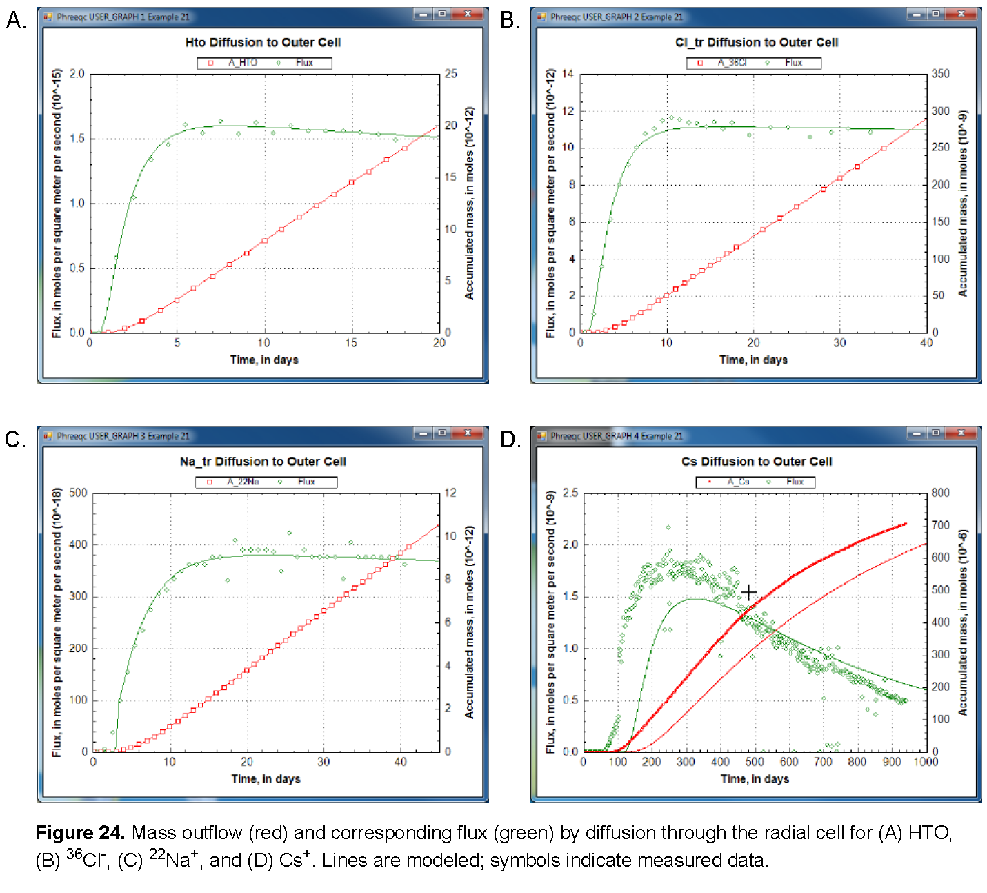
The model simulates the experimental results very well (fig. 24), except for Cs+. The calculated arrival time of Cs+ is almost 100 days later than observed and then the mass accumulates too slowly. This behavior of Cs+ has been found in many similar experiments. It has been modeled by increasing the diffusion coefficient and decreasing the sorption capacity for Cs+ relative to batch experiments; these adjustments can be easily incorporated in this example.
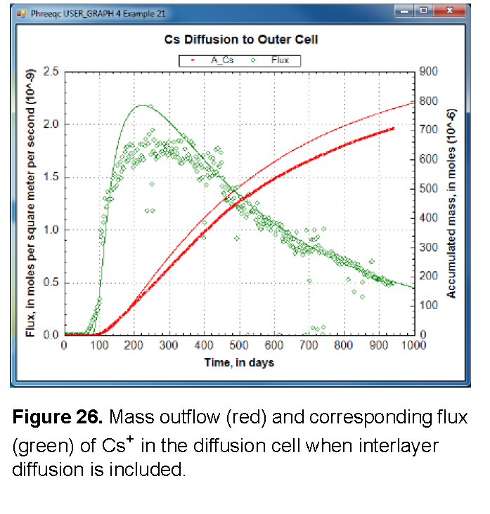
The diffusion of Cs+ can be increased by setting interlayer diffusion to true in Line 430:
430 interlayer_D$ = 'true'
(It is of interest to see the different effects of interlayer diffusion on 22Na+ and on Cs+.)
The results, shown in figure 26, illustrate that the arrival time of Cs+ can be matched by increasing diffusion, but that the mass accumulates too quickly. Another option for reducing the delay of the tracer arrival is to decrease the sorption of Cs+, either by decreasing the moles of surface and exchange sites or by decreasing the complexation constants, or both. By adjusting both the sorption and the diffusion coefficient, it may be possible to simulate the experimental data for Cs+. However, it remains difficult to explain why the sorption capacity is different between batch and diffusion experiments for Cs+, but not for the other cations.
Alternatively, and in line with the heterogeneous distribution of Cs+ in the clay after the experiment, the relatively fast arrival time can be modeled with a dual-porosity structure in which the pore space is subdivided into continuous and stagnant pores that can exchange by diffusion. The continuous pores allow Cs+ to move more rapidly through the clay than is calculated for a homogeneous medium, depending on the proportion, the flow velocity, and the diffusional exchange with the stagnant pores. With equation 49, and some effort, the dual-porosity structure can be introduced in the Basic program. Otherwise, the C program that is given as supplementary information in Appelo and others (2010) can be used. Similarly to the Basic program, the C program writes a complete PHREEQC input file for diffusion of Cs+, but in a dual porosity clay; in addition, the program permits distributing the surface and exchange sites differently between the stagnant and continuous pores.
 , (45)
 , and (46)