Table 44. Input file for example 15.
DATABASE ex15.dat
|
TITLE Example 15.--1D Transport: Kinetic Biodegradation, Cell Growth, and Sorption
|
***********
|
PLEASE NOTE: This problem requires database file ex15.dat!!
|
***********
|
PRINT
|
-reset false
|
-echo_input true
|
-status false
|
SOLUTION 0 Pulse solution with NTA and cobalt
|
units umol/L
|
pH 6
|
C .49
|
O(0) 62.5
|
Nta 5.23
|
Co 5.23
|
Na 1000
|
Cl 1000
|
SOLUTION 1-10 Background solution initially filling column
|
units umol/L
|
pH 6
|
C .49
|
O(0) 62.5
|
Na 1000
|
Cl 1000
|
COPY solution 0 100 # for use later on, and in
|
COPY solution 1 101 # 20 cells model
|
END
|
RATES Rate expressions for the four kinetic reactions
|
#
|
HNTA-2
|
-start
|
10 Ks = 7.64e-7
|
20 Ka = 6.25e-6
|
30 qm = 1.407e-3/3600
|
40 f1 = MOL("HNta-2")/(Ks + MOL("HNta-2"))
|
50 f2 = MOL("O2")/(Ka + MOL("O2"))
|
60 rate = -qm * KIN("Biomass") * f1 * f2
|
70 moles = rate * TIME
|
80 PUT(rate, 1) # save the rate for use in Biomass rate calculation
|
90 SAVE moles
|
-end
|
#
|
Biomass
|
-start
|
10 Y = 65.14
|
20 b = 0.00208/3600
|
30 rate = GET(1) # uses rate calculated in HTNA-2 rate calculation
|
40 rate = -Y*rate -b*M
|
50 moles = -rate * TIME
|
60 if (M + moles) < 0 then moles = -M
|
70 SAVE moles
|
-end
|
#
|
Co_sorption
|
-start
|
10 km = 1/3600
|
20 kd = 5.07e-3
|
30 solids = 3.75e3
|
40 rate = -km*(MOL("Co+2") - (M/solids)/kd)
|
50 moles = rate * TIME
|
60 if (M - moles) < 0 then moles = M
|
70 SAVE moles
|
-end
|
#
|
CoNta_sorption
|
-start
|
10 km = 1/3600
|
20 kd = 5.33e-4
|
30 solids = 3.75e3
|
40 rate = -km*(MOL("CoNta-") - (M/solids)/kd)
|
50 moles = rate * TIME
|
60 if (M - moles) < 0 then moles = M
|
70 SAVE moles
|
-end
|
KINETICS 1-10 Four kinetic reactions for all cells
|
HNTA-2
|
-formula C -3.12 H -1.968 O -4.848 N -0.424 Nta 1.
|
Biomass
|
-formula H 0.0
|
-m 1.36e-4
|
Co_sorption
|
-formula CoCl2
|
-m 0.0
|
-tol 1e-11
|
CoNta_sorption
|
-formula NaCoNta
|
-m 0.0
|
-tol 1e-11
|
COPY kinetics 1 101 # to use with 20 cells
|
END
|
SELECTED_OUTPUT
|
-file ex15.sel
|
-mol Nta-3 CoNta- HNta-2 Co+2
|
USER_PUNCH
|
-headings hours Co_sorb CoNta_sorb Biomass
|
-start
|
10 punch TOTAL_TIME/3600 + 3600/2/3600
|
20 punch KIN("Co_sorption")/3.75e3
|
30 punch KIN("CoNta_sorption")/3.75e3
|
40 punch KIN("Biomass")
|
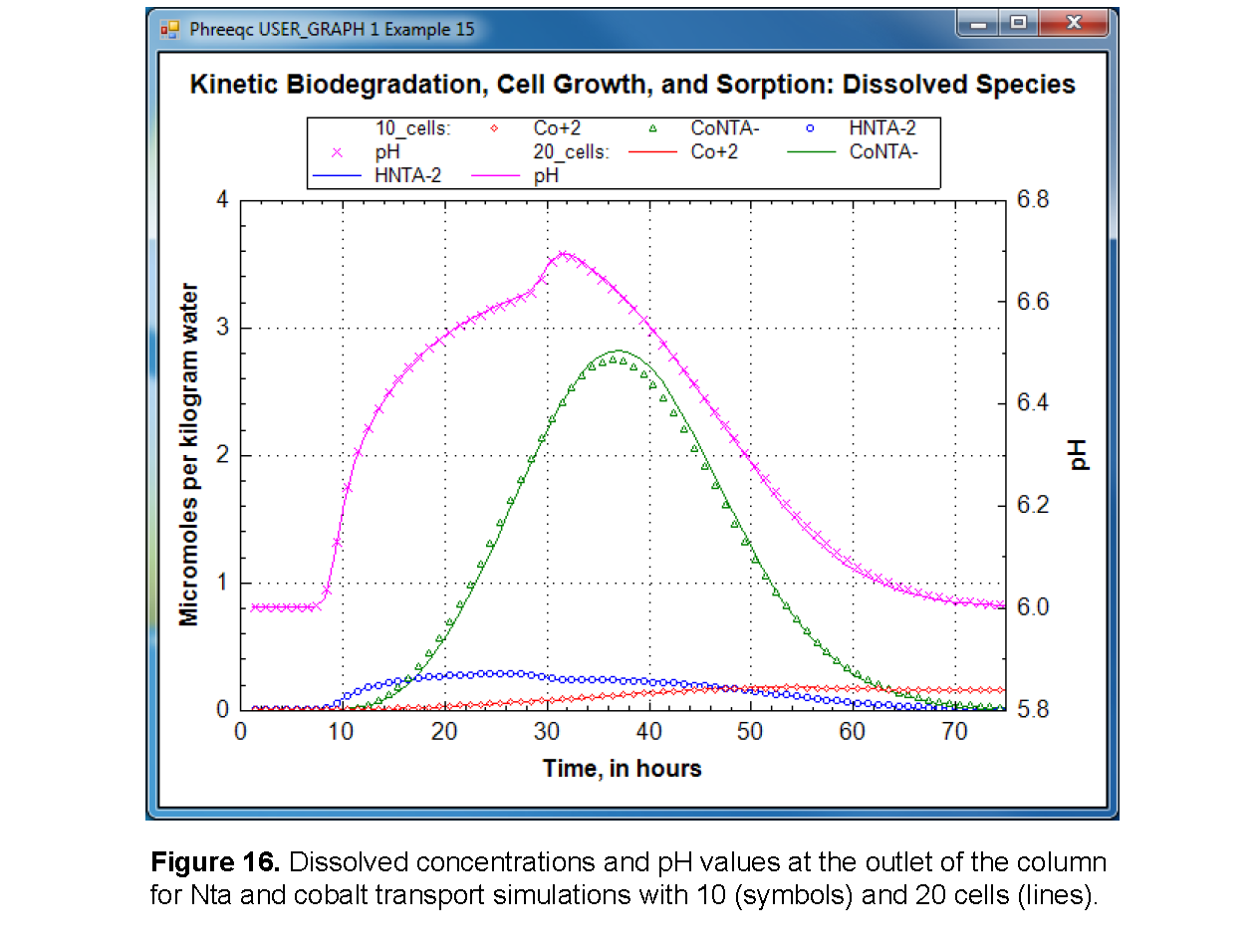
USER_GRAPH 1 Example 15
|
-headings 10_cells: Co+2 CoNTA- HNTA-2 pH
|
-chart_title "Kinetic Biodegradation, Cell Growth, and Sorption: Dissolved Species"
|
-axis_titles "Time, in hours" "Micromoles per kilogram water" "pH"
|
-axis_scale x_axis 0 75
|
-axis_scale y_axis 0 4
|
-axis_scale secondary_y_axis 5.799 6.8 0.2 0.1
|
-plot_concentration_vs t
|
-start
|
10 x = TOTAL_TIME/3600 + 3600/2/3600
|
20 PLOT_XY -1, -1, line_width = 0, symbol_size = 0
|
30 PLOT_XY x, MOL("Co+2") * 1e6, color = Red, line_width = 0, symbol_size = 4
|
40 PLOT_XY x, MOL("CoNta-") * 1e6, color = Green, line_width = 0, symbol_size = 4
|
50 PLOT_XY x, MOL("HNta-2") * 1e6, color = Blue, line_width = 0, symbol_size = 4
|
60 PLOT_XY x, -LA("H+"), y-axis = 2, color = Magenta, line_width = 0, symbol_size = 4
|
-end
|
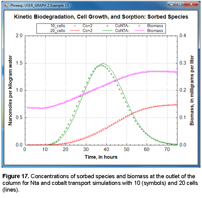
USER_GRAPH 2 Example 15
|
-headings 10_cells: Co+2 CoNTA- Biomass
|
-chart_title "Kinetic Biodegradation, Cell Growth, and Sorption: Sorbed Species"
|
-axis_titles "Time, in hours" "Nanomoles per kilogram water" \
|
"Biomass, in milligrams per liter"
|
-axis_scale x_axis 0 75
|
-axis_scale y_axis 0 2
|
-axis_scale secondary_y_axis 0 0.4
|
-plot_concentration_vs t
|
-start
|
10 x = TOTAL_TIME/3600 + 3600/2/3600
|
20 PLOT_XY -1, -1, line_width = 0, symbol_size = 0
|
30 PLOT_XY x, KIN("Co_sorption") / 3.75e3 * 1e9, color = Red, line_width = 0, symbol_size = 4
|
40 PLOT_XY x, KIN("CoNta_sorption") / 3.75e3 * 1e9, color = Green, line_width = 0, \
|
symbol_size = 4
|
50 PLOT_XY x, KIN("Biomass") * 1e3, y-axis = 2, color = Magenta, line_width = 0, \
|
symbol_size = 4
|
-end -end
|
TRANSPORT First 20 hours have NTA and cobalt in infilling solution
|
-cells 10
|
-lengths 1
|
-shifts 20
|
-time_step 3600
|
-flow_direction forward
|
-boundary_conditions flux flux
|
-dispersivities .05
|
-correct_disp true
|
-diffusion_coefficient 0.0
|
-punch_cells 10
|
-punch_frequency 1
|
-print_cells 10
|
-print_frequency 5
|
|
COPY solution 101 0 # initial column solution becomes influent
|
END
|
TRANSPORT Last 55 hours with background infilling solution
|
-shifts 55
|
COPY cell 100 0 # for the 20 cell model...
|
COPY cell 101 1-20
|
END
|
USER_PUNCH
|
-start
|
10 punch TOTAL_TIME/3600 + 3600/4/3600
|
20 punch KIN("Co_sorption")/3.75e3
|
30 punch KIN("CoNta_sorption")/3.75e3
|
40 punch KIN("Biomass")
|
-end
|
USER_GRAPH 1
|
-headings 20_cells: Co+2 CoNTA- HNTA-2 pH
|
-start
|
10 x = TOTAL_TIME/3600 + 3600/4/3600
|
20 PLOT_XY -1, -1, line_width = 0, symbol_size = 0
|
30 PLOT_XY x, MOL("Co+2") * 1e6, color = Red, symbol_size = 0
|
40 PLOT_XY x, MOL("CoNta-") * 1e6, color = Green, symbol_size = 0
|
50 PLOT_XY x, MOL("HNta-2") * 1e6, color = Blue, symbol_size = 0
|
60 PLOT_XY x, -LA("H+"), y-axis = 2, color = Magenta, symbol_size = 0
|
-end
|
USER_GRAPH 2
|
-headings 20_cells: Co+2 CoNTA- Biomass
|
-start
|
10 x = TOTAL_TIME/3600 + 3600/4/3600
|
20 PLOT_XY -1, -1, line_width = 0, symbol_size = 0
|
30 PLOT_XY x, KIN("Co_sorption") / 3.75e3 * 1e9, color = Red, symbol_size = 0
|
40 PLOT_XY x, KIN("CoNta_sorption") / 3.75e3 * 1e9, color = Green, symbol_size = 0
|
60 PLOT_XY x, KIN("Biomass") * 1e3, y-axis = 2, color = Magenta, symbol_size = 0
|
-end
|
TRANSPORT First 20 hours have NTA and cobalt in infilling solution
|
-cells 20
|
-lengths 0.5
|
-shifts 40
|
-initial_time 0
|
-time_step 1800
|
-flow_direction forward
|
-boundary_conditions flux flux
|
-dispersivities .05
|
-correct_disp true
|
-diffusion_coefficient 0.0
|
-punch_cells 20
|
-punch_frequency 2
|
-print_cells 20
|
-print_frequency 10
|
COPY cell 101 0
|
END
|
TRANSPORT Last 55 hours with background infilling solution
|
-shifts 110
|
END
|
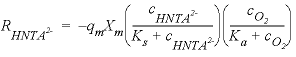 , (30)
 is the rate of HNta
2-
degradation (mol L
-1
h
-1
, mole per liter per hour),
is the rate of HNta
2-
degradation (mol L
-1
h
-1
, mole per liter per hour),  is the maximum specific rate of substrate utilization (mol/g cells/h),
  is the biomass (g L-1h-1, gram per liter per hour),
  is the half-saturation constant for the substrate Nta (mol/L),
  is the half-saturation constant for the electron acceptor O
2
(mol/L), and
c
indicates concentration (mol/L). The rate of biomass production is dependent on the rate of substrate utilization and a first-order decay rate for the biomass:
is the half-saturation constant for the electron acceptor O
2
(mol/L), and
c
indicates concentration (mol/L). The rate of biomass production is dependent on the rate of substrate utilization and a first-order decay rate for the biomass: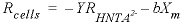 , (31)
 is the rate of cell growth (g L-1h-1),
Y
is the microbial yield coefficient (g cells/mol Nta), and
b
is the first-order biomass decay coefficient (h
-1
). The parameter values for these equations are listed in
is the rate of cell growth (g L-1h-1),
Y
is the microbial yield coefficient (g cells/mol Nta), and
b
is the first-order biomass decay coefficient (h
-1
). The parameter values for these equations are listed in  , (32)
 is the mass transfer coefficient (h
-1
), and
is the mass transfer coefficient (h
-1
), and  is the distribution coefficient (L/g, liter per gram). The values of the coefficients are given in