Example 20--Distribution of Isotopes Between Water and Calcite

The database iso.dat implements the approach to isotope reactions described by Thorstenson and Parkhurst (2002, 2004), in which minor isotopes are treated as individual thermodynamic components. The aqueous and solid species of minor isotopes have slightly different equilibrium constants than those of the major isotopes, which account for fractionation processes. The treatment of isotopes in gases requires a separate species for each isotopic variant of a gas; for example, the isotopic variants of carbon dioxide are CO2, C18OO, C18O2, 13CO2, 13C18OO, and 13C18O2. Similarly, every isotopic variant of a mineral must be included as a component of a solid solution to represent completely the isotopic composition of the solid. The equilibrium constants in iso.dat are derived from empirical fractionation factors, from statistical mechanical theory, or, where no data are available (the most common case), by assuming no fractionation. However, the database is a framework that can be expanded as additional isotopic thermodynamic data become available.

Example 20 considers the fractionation of oxygen-18, carbon-13, and carbon-14 between solution and calcite under two conditions: (1) in a system where a solution and isotopic solid solution equilibrate with sequential additions of calcite of a specified isotopic composition, hereafter referred to as marine calcite. This system is termed “closed” in the sense that all the masses of elements and isotopes that enter the system remain in the system; and (2) in a system where a solution and isotopic solid solution equilibrate with sequential additions of marine calcite, but the isotopic solid solution is removed from the system following equilibration. This system is termed “open” in the sense that masses of elements and isotopes are removed from the reaction system at each step. Both systems are isolated from the unsaturated zone, which precludes any further addition of carbon dioxide. The open system is equivalent to calculations in NETPATH that implement isotopic exchange, and the results of the PHREEQC open-system calculation are compared to NETPATH calculations for carbon-13 and carbon-14.

Example 20 is divided into two parts: first, the isotopic composition of a marine calcite solid solution in equilibrium with a solution of 0.0 permil oxygen-18 and 0.0 permil carbon-13 is estimated; second, the isotopic evolution of the solution and solid solution are calculated for the closed- and open-reaction systems. In addition to carbon-13 and oxygen-18, carbon-14 is included in the isotopic-evolution calculations, which allows carbon-14 to partition into the solid; however, the calculations do not consider the radioactive decay of carbon-14.

Calculation of the Composition of a Marine Calcite Isotopic Solid Solution

The input file that estimates the isotopic composition of calcite in equilibrium with a specified solution isotopic composition is given in table 57. The first line contains the DATABASE keyword and indicates that the iso.dat database file must be used for this calculation. The iso.dat database has thousands of aqueous species, many of which are negligibly small for most calculations. The PRINT data block is used to exclude species from the printed distribution of species for an element or isotope if the species concentration is less than a fraction of 10-6 relative to the total concentration of the element or isotope.

Table 57. Input file for example 20A.
DATABASE ../database/iso.dat
TITLE Example 20A.--Calculate carbonate solid solution
PRINT
-censor_species 1e-006
SOLUTION 1 # water to find composition of marine carbonate
pH 8.2
Na 1 charge
Ca 10 Calcite 0
C 2
[13C] 0 # permil
[14C] 0 # pmc
D 0 # permil
[18O] 0 # permil
END
SOLID_SOLUTION 1 No [14C]
Calcite
-comp Calcite 0
-comp CaCO2[18O](s) 0
-comp CaCO[18O]2(s) 0
-comp CaC[18O]3(s) 0
-comp Ca[13C]O3(s) 0
-comp Ca[13C]O2[18O](s) 0
-comp Ca[13C]O[18O]2(s) 0
-comp Ca[13C][18O]3(s) 0
END
RUN_CELLS
-cells 1
USER_PRINT
-start
10 PRINT pad("Component", 20), "Mole fraction"
20 t = LIST_S_S("Calcite", count, name$, moles)
30 for i = 1 to count
40 PRINT pad(name$(i),20), moles(i)/t
50 next i
-end
END

The SOLUTION data block defines an aqueous solution with isotopic composition of 0.0 permil carbon-13 and 0.0 permil oxygen-18, which are approximately the values in seawater. The solution contains dissolved inorganic carbon at a concentration of 2.0 mmol/kgw; the calcium concentration is determined by equilibrium (saturation index 0.0) with pure carbon-12, oxygen-16 calcite; and the sodium concentration is determined by charge balance. In the next simulation, a solid solution is defined that has eight components, but the number of moles of each component is zero. Thus, when reacting, components may precipitate, but no components initially are available to dissolve.

In the next simulation RUN_CELLS causes the solution and all of the reactants numbered 1 to react, namely SOLUTION 1 reacts with SOLID_SOLUTIONS 1. The solution is initially in equilibrium with a pure carbon-12, oxygen-16 calcite; however, a solid solution of all of the isotopic variants of calcite will be slightly less soluble than this pure solid. Thus, a solid solution should form, but the mole transfers to the solid should be small enough not to affect the isotopic composition of the solution substantially.

The composition of the isotopic solid solution is printed to the output file, but the printout only contains three significant digits. USER_PRINT is used to print the mole fractions with greater precision. The function LIST_S_S is used to retrieve the total number of moles of components (t, line 20) in the “Calcite” solid solution (as defined in SOLID_SOLUTIONS) and the name and number of moles of each component (name$ and moles, line 20). From these data, the mole fraction of each component is calculated and printed to the USER_PRINT section of the output file.

The mole fractions are interpreted as the number of moles of each component in a mole of the solid solution. The mole fractions calculated by the simulation are shown in table 58. The “Calcite” component represents the pure carbon-12, oxygen-16 component, which is approximately 98 percent of the solid; all other components are approximately 1 percent mole fraction or less.

“Calcite” is the name of the entire solid solution and also is the name of one of the components in the solid solution. Using “Calcite” for the solid solution name allows functions defined in iso.dat to be used to list isotope ratios and isotope alphas in the output file. The “Isotope Ratios” part of the printout (not shown) gives the isotopic compositions of the solution and the solid in terms of permil. The isotopic composition of oxygen-18 [R(18)] and carbon-13 [R(13)] in the solution are virtually unchanged from 0 permil. The oxygen-18 composition of the solid [R(18O) Calcite] is approximately 29 permil and the carbon-13 composition of the solid [R(13C) Calcite] is approximately 2 permil.

Table 58. Mole fractions of isotopic components in a marine carbonate solid solution.
Component Mole fraction
Calcite 9.8283e-001
Ca[13C]O3(s) 1.1011e-002
CaCO2[18O](s) 6.0825e-003
Ca[13C]O2[18O](s) 6.8147e-005
CaCO[18O]2(s) 1.2548e-005
Ca[13C]O[18O]2(s) 1.4058e-007
CaC[18O]3(s) 8.6284e-009
Ca[13C][18O]3(s) 9.6671e-011

Calculation of Open- and Closed-System Isotopic Evolution of Calcite and Solution

The concept for the isotope-evolution calculations is that water that has reacted with carbon dioxide in the unsaturated zone moves into the saturated zone and comes into contact with marine calcite with the composition defined by the previous calculation without further contact with carbon dioxide gas. The marine calcite reacts incrementally with the solution (0.0005 mol per increment), and after a few increments, a solid solution forms. In the open-system calculation, the solution moves on to react with pristine marine calcite, leaving the previously formed solid solution behind. In the closed system, the entire system--previously formed solid solution, increment of marine calcite, and solution--reacts to a new equilibrium. Although the isotopic compositions of the unsaturated zone solution are substantially different from the marine calcite, with sufficient reaction of the marine calcite, the solution will ultimately approach a composition that is in equilibrium with the pure marine calcite for both the open- and closed-system paths.

The input file for the open- and closed-system calculations is given in table 59. As in the previous calculations, iso.dat is used as the database and the species concentrations printed in the distribution of species are censored at 10^-6 . Carbon-14 is included in the calculations, which results in very small concentrations of carbon-14 atoms in solution. These small concentrations can lead to instabilities in the numerical method used to solve the constitutive equations. The KNOBS data block sets a smaller step size and an alternative equation scaling than the default, which helps in the solution of the equations. Alternatively, results are linear for such small concentrations of carbon-14, and a larger concentration of carbon-14 (say 10 or 100 times larger) could be used to increase numerical stability, provided the results are reduced in the same proportion.

Table 59. Input file for example 20B.
DATABASE ../database/iso.dat
TITLE Example 20B.--Isotope evolution.
PRINT
-censor_species 1e-006
KNOBS
-diagonal_scale
-step 10
-pe 5
#
# Open system calculation
#
SOLID_SOLUTION 1 With [14C]
Calcite
-comp Calcite 0
-comp CaCO2[18O](s) 0
-comp CaCO[18O]2(s) 0
-comp CaC[18O]3(s) 0
-comp Ca[13C]O3(s) 0
-comp Ca[13C]O2[18O](s) 0
-comp Ca[13C]O[18O]2(s) 0
-comp Ca[13C][18O]3(s) 0
-comp Ca[14C]O3(s) 0
-comp Ca[14C]O2[18O](s) 0
-comp Ca[14C]O[18O]2(s) 0
-comp Ca[14C][18O]3(s) 0
END
REACTION 1
Calcite 9.8283e-001
Ca[13C]O3(s) 1.1011e-002
CaCO2[18O](s) 6.0825e-003
Ca[13C]O2[18O](s) 6.8147e-005
CaCO[18O]2(s) 1.2548e-005
Ca[13C]O[18O]2(s) 1.4058e-007
CaC[18O]3(s) 8.6284e-009
Ca[13C][18O]3(s) 9.6671e-011
0.0005 mole
END
USER_PRINT
10 PRINT "Calcite added: ", GET(0) * RXN
USER_GRAPH 1 Example 20
-headings Open--Dissolved Open--Calcite
-chart_title "Oxygen-18"
-axis_titles "Marine calcite reacted, in moles" "Permil"
-axis_scale x_axis 0 0.05 a a
-axis_scale y_axis -10 30 a a
-start
10 PUT(GET(0) + 1, 0)
20 PLOT_XY RXN*GET(0),ISO("R(18O)"), color=Red, line_w=2, symbol=None
30 PLOT_XY RXN*GET(0),ISO("R(18O)_Calcite"), color=Green, line_w=2, symbol=None
-end
END
USER_GRAPH 2 Example 20
-headings Open--Dissolved Open-Calcite
-chart_title "Carbon-13"
-axis_titles "Marine calcite reacted, in moles" "Permil"
-axis_scale x_axis 0 0.05 a a
-axis_scale y_axis -25 5.0 a a
-plot_tsv ex20-c13.tsv
-start
10 PLOT_XY RXN*GET(0),ISO("R(13C)"), color=Red, line_w=2, symbol=None
20 PLOT_XY RXN*GET(0),ISO("R(13C)_Calcite"), color=Green, line_w=2, symbol=None
-end
END
USER_GRAPH 3 Example 20
-headings Open--Dissolved Open--Calcite
-chart_title "Carbon-14"
-axis_titles "Marine calcite reacted, in moles" "Percent modern carbon"
-axis_scale x_axis 0 0.05 a a
-axis_scale y_axis 0 100 a a
-plot_tsv ex20-c14.tsv
-start
10 PLOT_XY RXN*GET(0),ISO("R(14C)"), color=Red, line_w=2, symbol=None
20 PLOT_XY RXN*GET(0),ISO("R(14C)_Calcite"), color=Green, line_w=2, symbol=None
-end
END
SOLUTION 1
pH 5 charge
pe 10
C 2 CO2(g) -1.0
[13C] -25 # permil
[14C] 100 # pmc
[18O] -5 # permil
SELECTED_OUTPUT
-reset false
-file ex20_open
USER_PUNCH
-start
10 FOR i = 1 to 100
20 PUNCH EOL$ + "USE solution 1"
30 PUNCH EOL$ + "USE solid_solution 1"
40 PUNCH EOL$ + "USE reaction 1"
50 PUNCH EOL$ + "SAVE solution 1"
60 PUNCH EOL$ + "END"
70 NEXT i
-end
END
PRINT
-selected_output false
END
INCLUDE$ ex20_open
END
#
# Closed system calculation
#
USER_GRAPH 1 Oxygen-18
-headings Closed--Dissolved Closed--Calcite
-start
10 PUT(GET(1) + 1, 1)
20 PLOT_XY RXN*GET(1),ISO("R(18O)"), color=Blue, line_w=0, symbol=Circle
30 PLOT_XY RXN*GET(1),ISO("R(18O)_Calcite"), color=Black, line_w=0, symbol=Circle
-end
END
USER_GRAPH 2 Carbon-13
-headings Closed--Dissolved Closed--Calcite
-start
10 PLOT_XY RXN*GET(1),ISO("R(13C)"), color=Blue, line_w=2, symbol=None
20 PLOT_XY RXN*GET(1),ISO("R(13C)_Calcite"), color=Black, line_w=2, symbol=None
-end
END
USER_GRAPH 3 Carbon-14
-headings Closed--Dissolved Closed--Calcite
-start
10 PLOT_XY RXN*GET(1),ISO("R(14C)"), color=Blue, line_w=2, symbol=None
20 PLOT_XY RXN*GET(1),ISO("R(14C)_Calcite"), color=Black, line_w=2, symbol=None
-end
END
USER_PRINT
10 PRINT "Calcite added: ", GET(1), GET(1)*0.0005, RXN
SOLUTION 1
pH 5 charge
pe 10
C 2 CO2(g) -1.0
[13C] -25 # permil
[14C] 100 # pmc
[18O] -5 # permil
END
INCREMENTAL_REACTIONS true
# Alternative to redefinition of REACTION 1
#REACTION_MODIFY 1
# -steps
# 0.05
# -equal_increments 1
# -count_steps 100
REACTION 1
Calcite 9.8283e-001
Ca[13C]O3(s) 1.1011e-002
CaCO2[18O](s) 6.0825e-003
Ca[13C]O2[18O](s) 6.8147e-005
CaCO[18O]2(s) 1.2548e-005
Ca[13C]O[18O]2(s) 1.4058e-007
CaC[18O]3(s) 8.6284e-009
Ca[13C][18O]3(s) 9.6671e-011
0.05 mole in 100 steps
RUN_CELLS
-cells 1
END

As in the previous calculation, a solid solution with zero moles of components is defined in the SOLID_SOLUTIONS data block; however, this time, four carbon-14 solid components also are defined. A reaction is defined by using the composition of the calcite isotopic solid solution of the previous calculation. The components are present in the proportions given by the mole fractions, but the reaction adds only 0.0005 mol of marine calcite per increment. Next, three USER_GRAPH data blocks are defined to display the isotopic composition of oxygen-18, carbon-13, and carbon-14 in the solid and in solution as the reactions proceed.

The SOLUTION definition represents an unsaturated zone water. The carbon concentration is determined by equilibrium with a soil-zone partial pressure of 0.1 atm for carbon dioxide gas. Carbon-13 is set to -25 permil to represent an organic matter source of the carbon dioxide. Carbon-14 of the soil gas is assumed to be 100 pmc. Oxygen-18 is arbitrarily set to -5 permil, which is typical of a temperate climate.

The open-system simulation requires a series of calculations where an increment of marine calcite is added to the solution and equilibrated with a solid solution, followed by saving the solution composition. This sequence is repeated 100 times. It is possible to use an editor to create the input file by cutting and pasting 100 copies of the sequence of statements. For compactness, USER_PUNCH is used to write 100 copies of the sequence into the file ex20_open, which is then included in the input file with an INCLUDE$ statement. The PRINT data block (or a new definition of USER_PUNCH) is necessary to avoid repeatedly writing USER_PUNCH output to file for each subsequent calculation.

The closed-system calculation is similar to the open-system calculation. USER_GRAPH data blocks are used to set the parameters for the closed-system plots, which will be added to the open-system plots. The initial unsaturated-zone water is redefined with SOLUTION. However, in the closed system, the compositions of both the solution and the solid solution need to be saved after each increment. By saving the compositions at each reaction step, the closed-system definition is actually much simpler than the open system definition. The reaction can be defined as 0.05 mol in 100 steps, and RUN_CELLS can be used to bring together all the reactants numbered 1 (REACTION 1, SOLUTION 1, and SOLID_SOLUTIONS 1) for the series of 100 calculations. RUN_CELLS automatically saves the compositions of all reactants after each reaction step.

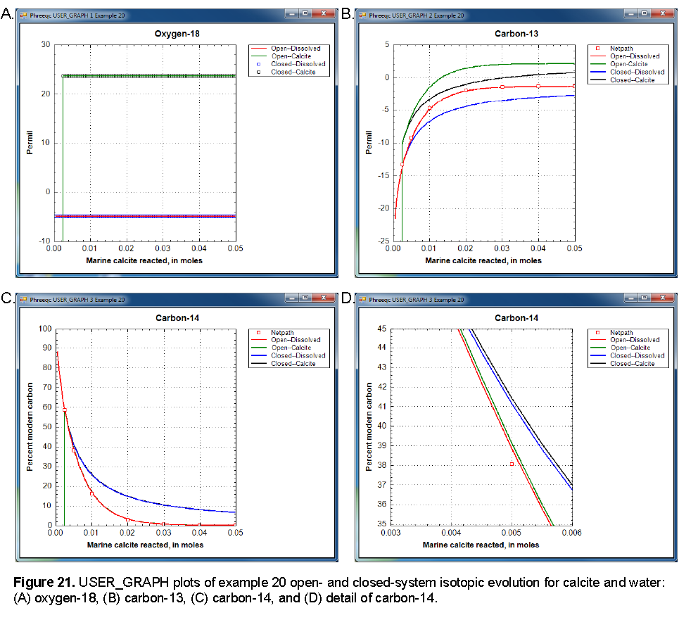
The isotopic compositions of the open and closed systems as a function of marine calcite reacted are shown in figure 21. The isotopic compositions begin at the composition of the unsaturated-zone water. Initially, the water is undersaturated with the isotopic solid solution and no solid is present. The vertical lines on panels A, B, and C indicate the point at which a solid solution begins to form.

Oxygen-18 is essentially constant in the water and solid through the course of the reactions because the water phase dominates. There are 55.5 mol of oxygen in the water, whereas only 0.05 mol of marine calcite react. Thus, oxygen-18 in the water remains essentially equal to the initial composition of -5.0 permil, although, in detail, there is a slight trend to heavier compositions. The isotopic solid solution in equilibrium with the water is approximately 24 permil. Open- and closed-system calculations give identical results for oxygen-18.

As more and more marine calcite reacts, the carbon-13 isotopic composition of the solid approaches 2 permil, which is the composition of the marine calcite (fig. 21, panel B). The open system approaches the value more quickly than the closed system because only the isotopes in the water are carried forward to the next step and the solid solution (containing some of the lighter isotopes) is left behind. In the closed system, more reaction is needed to approach the marine calcite composition because all the light isotopes from the initial solution remain in the system and must be diluted by more heavy isotopes from the marine calcite. The carbon in the water is about 3.5 permil lighter than the carbon in the solid solution for both the open- and closed-system calculations.

Initially, all carbon-14 is in the unsaturated-zone water. As marine calcite reacts, the carbon-14 partitions into the solid and asymptotically approaches the point when all carbon-14 is in the solid solution. As with carbon-13, the open-system calculation approaches this point more quickly than the closed system calculation. Fractionation does occur for carbon-14 as it does for carbon-13; the detailed plot in figure 21, panel D, shows that the solid solution is slightly heavier than the solution, but the effect is insignificantly small. Radioactive decay of carbon-14 has been ignored in these calculations; all of the effects of decreasing carbon-14 concentrations in these calculations are the result of partitioning carbon-14 into the solid. If the rate of partitioning carbon-14 into solids is fast relative to the half-life of carbon-14 (approximately 6,000 yr), then it would be an important consideration in carbon-14 groundwater dating. If substantial loss of carbon-14 to the solid were erroneously attributed to radioactive decay, the resulting groundwater ages would be too old.

NETPATH was used to model the effects of isotopic exchange with the marine calcite on the evolution of carbon-13 and carbon-14 from the point that the solid solution forms. The fractionation factors of Deines and others (1974) are used in the iso.dat database and, consequently, the Deines option in NETPATH was used to maintain consistency in the calculations. NETPATH uses an analytical solution to the fractionation equations, whereas PHREEQC calculations used numerical integration with 0.0005 mole reaction steps. NETPATH results and PHREEQC results are very similar (fig. 21, panels B and C), which indicates both that the isotopic approach in PHREEQC is workable and that the reactions steps were sufficiently small to obtain accurate results.