| Next || Previous || Top |
Example 2--Equilibration With Pure Phases
This example shows how to calculate the solubility and relative thermodynamic stability of two minerals, gypsum and anhydrite. First, as a function of temperature at 1 atm, and second, as a function of temperature and pressure, while comparing the calculations with experimental solubility data.
Conceptually, the two models define a beaker with pure water to which the minerals gypsum and (or) anhydrite are added. Step-wise, the beaker is heated, the minerals dissolve to equilibrium, and the concentrations and saturation indexes are calculated and plotted. If, at a given temperature, gypsum is less soluble than anhydrite, anhydrite dissolves completely while gypsum precipitates; similarly, if gypsum is more soluble than anhydrite, anhydrite dissolves completely and gypsum precipitates. Adding a single mineral allows the (possibly metastable) solubility at any temperature and pressure to be calculated.
The input file for the first model is given in table 12. It defines a single simulation in which various keywords define the actions that will be processed together. The water is defined with keyword SOLUTION. It is given a pH of 7 and a temperature of 25 °C, but these are equal to default and could be omitted. Also, by default, the pe is 4 and the density is 1 kg/L, and by omitting these parameters the default values will be used. The two minerals are defined with keyword EQUILIBRIUM_PHASES. The mineral name is followed by the target saturation index and the amount in moles (defaults are 0 and 10, respectively). If a phase is not present initially, it can be given 0 mol. Of course, the mineral names must have been defined before through a PHASES data block in the database or the input file. The REACTION_TEMPERATURE data block lets the temperature change from 25 °C to 75 °C in 51 steps (25, 26, ..., 75 °C).
Table 12. Input file for example 2.
TITLE Example 2.--Temperature dependence of solubility
|
of gypsum and anhydrite
|
SOLUTION 1 Pure water
|
pH 7.0
|
temp 25.0
|
EQUILIBRIUM_PHASES 1
|
Gypsum 0.0 1.0
|
Anhydrite 0.0 1.0
|
REACTION_TEMPERATURE 1
|
25.0 75.0 in 51 steps
|
SELECTED_OUTPUT
|
-file ex2.sel
|
-temperature
|
-si anhydrite gypsum
|
USER_GRAPH 1 Example 2
|
-headings Temperature Gypsum Anhydrite
|
-chart_title "Gypsum-Anhydrite Stability"
|
-axis_scale x_axis 25 75 5 0
|
-axis_scale y_axis auto 0.05 0.1
|
-axis_titles "Temperature, in degrees celsius" "Saturation index"
|
-initial_solutions false
|
-start
|
10 graph_x TC
|
20 graph_y SI("Gypsum") SI("Anhydrite")
|
-end
|
END
|
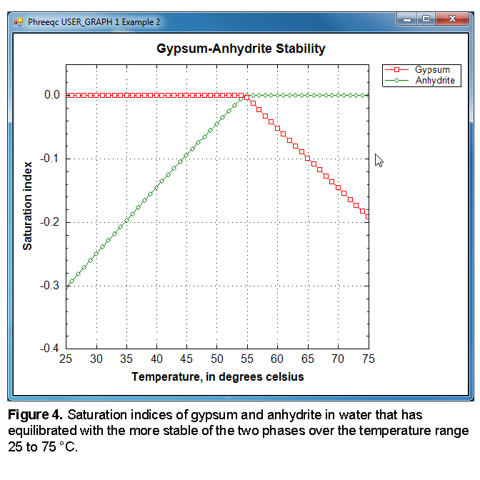
At each step, the temperature and the saturation indices for gypsum and anhydrite are written to the file
ex2.sel
as defined by SELECTED_OUTPUT, and plotted by USER_GRAPH as shown in figure 4. The figure shows that below 58 °C, the solution is in equilibrium with gypsum, but subsaturated with respect to anhydrite. Above that temperature, anhydrite is the more stable phase.
PHREEQC starts the simulation by calculating the solution composition if a new SOLUTION (or SOLUTION_SPREAD) data block is defined, continues with the reactions defined with the keywords, and prints the results of the calculations. The printout of the initial solution and the first batch-reaction step is listed in table 13. Headings define the various parts and are self-explanatory.
Table 13. Selected output for example 2.
-------------------------------------------
|
Beginning of initial solution calculations.
|
-------------------------------------------
|
|
Initial solution 1. Pure water
|
|
-----------------------------Solution composition------------------------------
|
|
Elements Molality Moles
|
|
Pure water
|
|
----------------------------Description of solution----------------------------
|
|
pH = 7.000
|
pe = 4.000
|
Specific Conductance (uS/cm, 25 oC) = 0
|
Density (g/cm3) = 0.99704
|
Volume (L) = 1.00297
|
Activity of water = 1.000
|
Ionic strength = 1.007e-007
|
Mass of water (kg) = 1.000e+000
|
Total alkalinity (eq/kg) = 1.217e-009
|
Total carbon (mol/kg) = 0.000e+000
|
Total CO2 (mol/kg) = 0.000e+000
|
Temperature (deg C) = 25.00
|
Electrical balance (eq) = -1.217e-009
|
Percent error, 100*(Cat-|An|)/(Cat+|An|) = -0.60
|
Iterations = 0
|
Total H = 1.110124e+002
|
Total O = 5.550622e+001
|
|
----------------------------Distribution of species----------------------------
|
|
Log Log Log mole V
|
Species Molality Activity Molality Activity Gamma cm3/mol
|
|
OH- 1.013e-007 1.012e-007 -6.995 -6.995 -0.000 -4.14
|
H+ 1.001e-007 1.000e-007 -7.000 -7.000 -0.000 0.00
|
H2O 5.551e+001 1.000e+000 1.744 0.000 0.000 18.07
|
H(0) 1.416e-025
|
H2 7.079e-026 7.079e-026 -25.150 -25.150 0.000 28.61
|
O(0) 0.000e+000
|
O2 0.000e+000 0.000e+000 -42.080 -42.080 0.000 30.40
|
|
------------------------------Saturation indices-------------------------------
|
|
Phase SI log IAP log K(298 K, 1 atm)
|
|
H2(g) -22.05 -25.15 -3.10 H2
|
H2O(g) -1.50 0.00 1.50 H2O
|
O2(g) -39.19 -42.08 -2.89 O2
|
|
|
-----------------------------------------
|
Beginning of batch-reaction calculations.
|
-----------------------------------------
|
|
Reaction step 1.
|
|
Using solution 1. Pure water
|
Using pure phase assemblage 1.
|
Using temperature 1.
|
|
-------------------------------Phase assemblage--------------------------------
|
|
Moles in assemblage
|
Phase SI log IAP log K(T, P) Initial Final Delta
|
|
Anhydrite -0.30 -4.58 -4.28 1.000e+000 0 -1.000e+000
|
Gypsum 0.00 -4.58 -4.58 1.000e+000 1.985e+000 9.855e-001
|
|
-----------------------------Solution composition------------------------------
|
|
Elements Molality Moles
|
|
Ca 1.508e-002 1.455e-002
|
S 1.508e-002 1.455e-002
|
|
----------------------------Description of solution----------------------------
|
|
pH = 7.066 Charge balance
|
pe = 10.745 Adjusted to redox equilibrium
|
Specific Conductance (uS/cm, 25 oC) = 2161
|
Density (g/cm3) = 0.99909
|
Volume (L) = 0.96829
|
Activity of water = 1.000
|
Ionic strength = 4.183e-002
|
Mass of water (kg) = 9.645e-001
|
Total alkalinity (eq/kg) = 1.261e-009
|
Total carbon (mol/kg) = 0.000e+000
|
Total CO2 (mol/kg) = 0.000e+000
|
Temperature (deg C) = 25.00
|
Electrical balance (eq) = -1.217e-009
|
Percent error, 100*(Cat-|An|)/(Cat+|An|) = -0.00
|
Iterations = 19
|
Total H = 1.070706e+002
|
Total O = 5.359351e+001
|
|
----------------------------Distribution of species----------------------------
|
|
Log Log Log mole V
|
Species Molality Activity Molality Activity Gamma cm3/mol
|
|
OH- 1.431e-007 1.178e-007 -6.844 -6.929 -0.084 -3.90
|
H+ 9.974e-008 8.587e-008 -7.001 -7.066 -0.065 0.00
|
H2O 5.551e+001 9.996e-001 1.744 -0.000 0.000 18.07
|
Ca 1.508e-002
|
Ca+2 1.046e-002 5.176e-003 -1.981 -2.286 -0.305 -17.66
|
CaSO4 4.627e-003 4.672e-003 -2.335 -2.331 0.004 7.50
|
CaOH+ 1.203e-008 1.000e-008 -7.920 -8.000 -0.080 (0)
|
CaHSO4+ 3.172e-009 2.637e-009 -8.499 -8.579 -0.080 (0)
|
H(0) 3.354e-039
|
H2 1.677e-039 1.693e-039 -38.776 -38.771 0.004 28.61
|
O(0) 2.878e-015
|
O2 1.439e-015 1.453e-015 -14.842 -14.838 0.004 30.40
|
S(-2) 0.000e+000
|
HS- 0.000e+000 0.000e+000 -118.111 -118.195 -0.084 20.77
|
H2S 0.000e+000 0.000e+000 -118.324 -118.320 0.004 37.16
|
S-2 0.000e+000 0.000e+000 -123.735 -124.047 -0.312 (0)
|
S(6) 1.508e-002
|
SO4-2 1.046e-002 5.075e-003 -1.981 -2.295 -0.314 14.66
|
CaSO4 4.627e-003 4.672e-003 -2.335 -2.331 0.004 7.50
|
HSO4- 5.096e-008 4.237e-008 -7.293 -7.373 -0.080 40.44
|
CaHSO4+ 3.172e-009 2.637e-009 -8.499 -8.579 -0.080 (0)
|
|
------------------------------Saturation indices-------------------------------
|
|
Phase SI log IAP log K(298 K, 1 atm)
|
|
Anhydrite -0.30 -4.58 -4.28 CaSO4
|
Gypsum 0.00 -4.58 -4.58 CaSO4:2H2O
|
H2(g) -35.67 -38.77 -3.10 H2
|
H2O(g) -1.50 -0.00 1.50 H2O
|
H2S(g) -117.27 -125.26 -7.99 H2S
|
O2(g) -11.95 -14.84 -2.89 O2
|
Sulfur -87.58 -82.70 4.88 S
|
The heading “Phase assemblage” records the saturation indices and amounts of each of the phases defined by EQUILIBRIUM_PHASES. In the first batch-reaction step, the solution is undersaturated with respect to anhydrite (saturation index is -0.30), and in equilibrium with gypsum (saturation index is 0.0). Consequently, all of the anhydrite has dissolved and most of the calcium and sulfate have precipitated as gypsum. The “Solution composition” shows that 15.1 mmol/kgw of calcium and sulfate are in solution, which is the solubility of gypsum in pure water at 25 °C. However, the total moles of the two constituents in the aqueous phase is only 14.6 because the mass of water has decreased to 0.964 kg by precipitating gypsum (CaSO4
.
2H2O), as printed below “Description of solution”. Accordingly, the mass of solvent water is not constant in batch-reaction calculations because reactions and waters of hydration in dissolving and precipitating phases may increase or decrease the mass of solvent water. Also listed under “Description of solution” are the calculated specific conductance (2161 μS/cm, microsiemens per centimeter), the density (0.999 g/cm
3
), the cation-anion balance (0), and more.
To illustrate that the temperature where gypsum transforms into anhydrite is a function of pressure, the calculation is repeated with input file ex2b at pressures of 1, 500, and 1,000 bars. The calculated results are compared with experimental data summarized by Blount and Dickson (1973, figure 2). Part of the input file is listed in table 14.
Table 14. Input file for the first and second simulation in example 2B.
TITLE Calculate gypsum/anhydrite transitions, 30 - 170 oC, 1 - 1000 atm
|
Data in ex2b.tsv from Blount and Dickson, 1973, Am. Mineral. 58, 323, fig. 2.
|
PRINT; -reset false
|
SOLUTION 1
|
EQUILIBRIUM_PHASES
|
Gypsum
|
REACTION_TEMPERATURE
|
30 90 in 10
|
USER_GRAPH 1 Example 2B, (P, T)-dependent solubilities of Gypsum and Anhydrite
|
-plot_tsv_file ex2b.tsv
|
-axis_titles "Temperature, in degrees celsius" "Solubility, in moles per \
|
kilogram water"
|
-axis_scale x_axis 30 170
|
-axis_scale y_axis 1e-3 0.05 auto auto log
|
10 plot_xy tc, tot("Ca"), color = Red, symbol = None
|
-end
|
END # 1st simulation
|
|
USE solution 1
|
USE equilibrium_phases 1
|
USE reaction_temperature 1
|
REACTION_PRESSURE 2
|
493
|
USER_GRAPH
|
10 plot_xy tc, tot("Ca"), color = Red, symbol = None
|
END
|
|
USE solution 1
|
USE equilibrium_phases 1
|
USE reaction_temperature 1
|
REACTION_PRESSURE 3
|
987
|
USER_GRAPH
|
20 plot_xy tc, tot("Ca"), color = Red, symbol = None
|
END # 2nd simulation
|
Like before in table 13 (example file ex2 in the PHREEQC distribution), the first simulation of table 14 (example file ex2b in the PHREEQC distribution) defines the SOLUTION, the EQUILIBRIUM_PHASES, the REACTION_TEMPERATUREs, and USER_GRAPH for plotting the experimental solubilities from file ex2b.tsv and the calculated concentrations. To accelerate the calculations, the output is reduced by using PRINT;
-reset false
. The second simulation of table 14 uses the same definitions through the USE data blocks and defines the reaction pressure as 493 atmospheres (= 500 bar). The third simulation in ex2b (not listed in table 14) does the same for 1,000 bars, and further simulations repeat the calculations with anhydrite as the equilibrium phase.
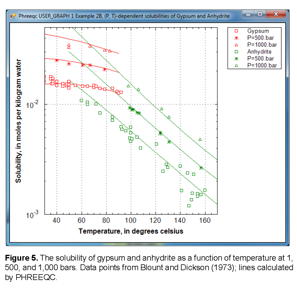
Figure 5 shows the solubility (note the logarithmic scale) as a function of temperature. The temperature of the gypsum to anhydrite transition increases from 58 °C at 1 atm, to 63 °C at 493 atm (= 500 bar), and 70 °C at 987 atm (= 1,000 bar). Thus, the stability of gypsum relative to anhydrite increases with pressure, which is because water in the gypsum crystal has a smaller volume than water in solution:
CaSO4∙2H2O = CaSO4 + 2H2O.
However, as illustrated in figure 5, the solubility of gypsum increases with pressure because the sum of the aqueous molar volumes of the solute species together is smaller than the molar volume of gypsum. Another point to note is that the experimental data for the gypsum solubility extend into the stability field of anhydrite. Apparently, the precipitation of anhydrite is too slow to reduce the concentrations in the experiments.
| Next || Previous || Top |