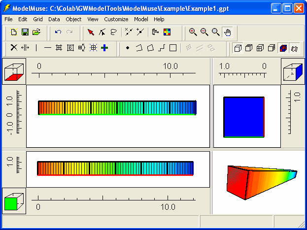
21.The model is now ready to execute. However, before executing it, it is worthwhile to color the grid with some of the data sets to make sure the data have been applied properly. Select Data|Color Grid… and select the Initial_Head data set (under Data Sets|Required|Hydrology) . Click the Apply button. The model should appear similar to figure 49. Try using the Selection Cube for the side view of the model to change the selected column progressively from 1 to 61. The color displayed on the side view should change from red to blue. (See the Selection Cube.) If the mouse cursor is over a colored cell or element on the top view of the model, the value of the data set for the colored element or cell will be displayed in the third panel of the status bar along with an explanation of how the value was assigned. It is possible to color the grid using the Specified_Head_Solution boundary condition at time 0 and time 60.

Figure 49. Main window showing the grid being colored by the Initial_Head data set.
22.Now that the model has been set up, it is possible to execute it. First copy phast.dat and ex1.chem.dat from the examples distributed with PHAST to the location where ex1.trans.dat will be saved. Then select File|Export|PHAST Input File. In the Save File dialog box make sure the Execute model checkbox is checked and save the file as ex1.trans.dat. When it is finished executing, Model Viewer (Hsieh and Winston, 2002) can be used to display the results. (The capability of displaying PHAST results in Model Viewer was added by Scott R. Charlton.)