Seepage Face

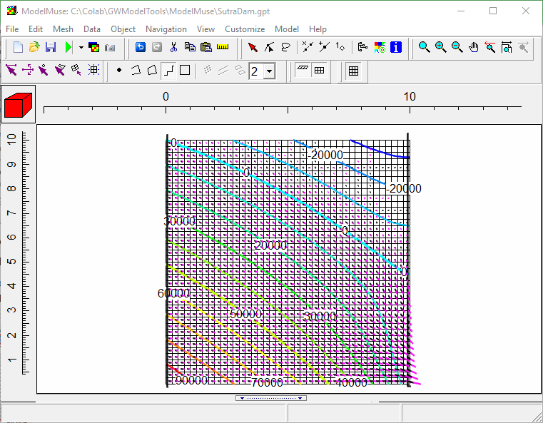
This example approximately reproduces the seepage face example from page 14 of the SUTRA 3.0 documentation. It uses the Generalized-Flow boundary. Please read that section to better understand this example.

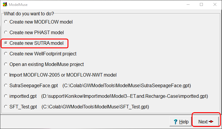
Start by creating a new SUTRA model.

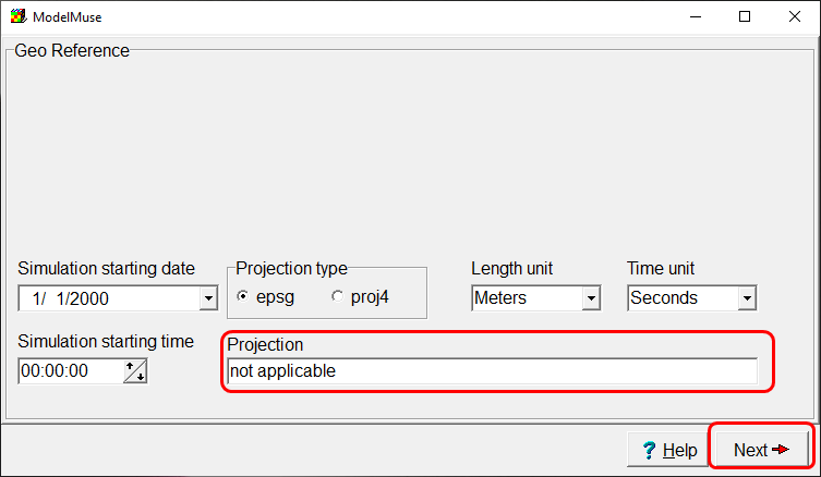
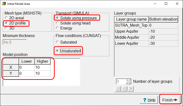
Set the model as a 2D profile model using using pressure and unsaturated. The model will end up being 10 meters wide and high so set the lower position of X and Y to 0 and the higher position to 10. Then click the "Finish" button.

Select View|Vertical Exaggeration and set the vertical exaggeration to 1.

We will use the fishnet mesh tools to create a mesh exactly 10 meters wide and high with square elements that have edges 0.25 meters long. Click the Draw fishnet mesh quadrilaterals button and click in the main window to outline an area approximately 10 m wide by 10 meters high. When you are done, double click inside the quadrilateral and set the four corners of the quadrilateral to (0, 0), (0,10), (10,10), and (10,0).

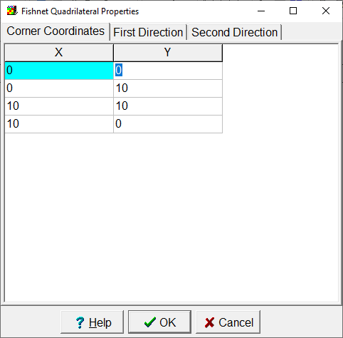
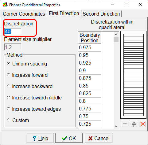
Set the discretization to 40 for both the first and second directions.

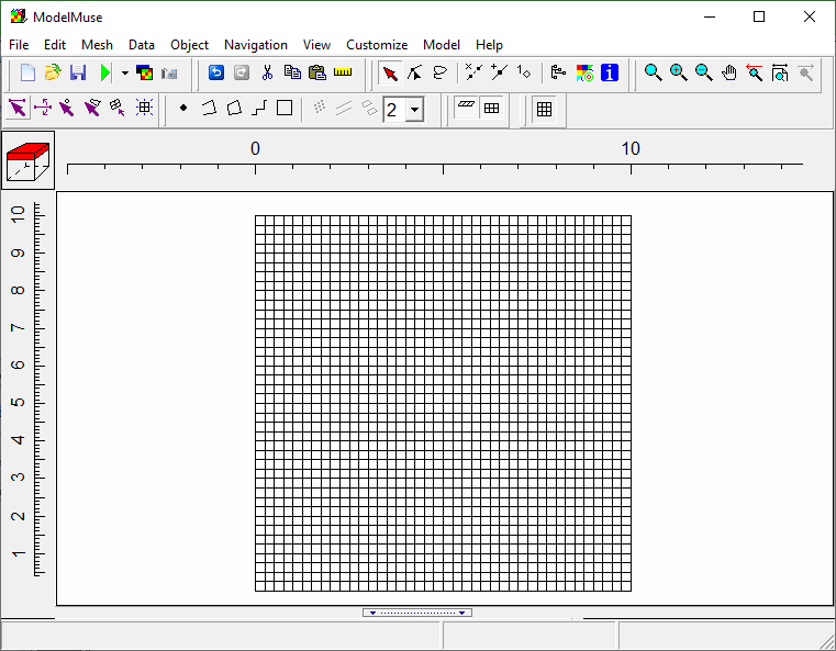
Click the Generate Mesh button and then click the OK button to generate the mesh.

Next we will set the options for the model. Select Model|SUTRA Options.

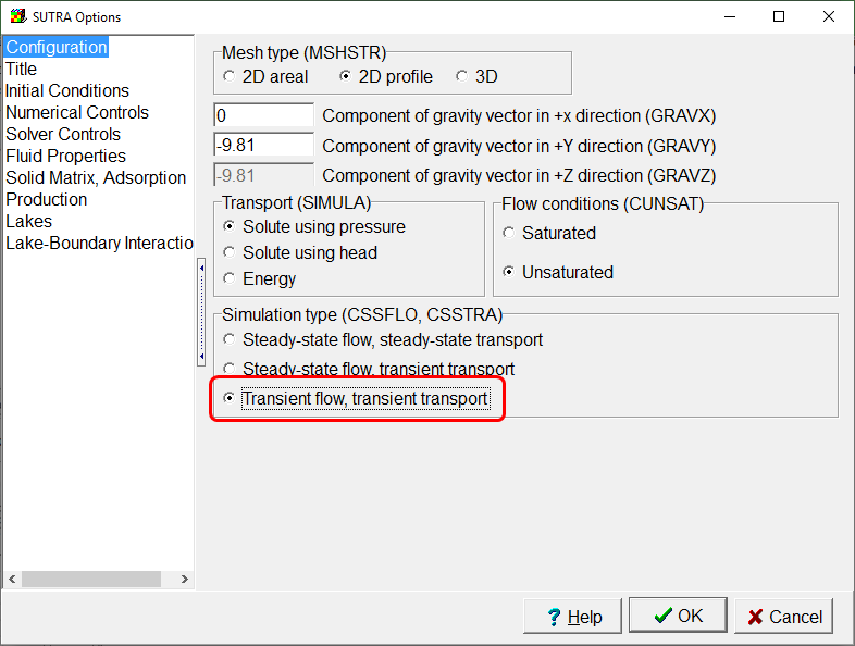
On the Configuration tab, set the simulation type to Transient flow, transient transport.

Enter the following text on the title tab. "Dam example: Demonstrates generalized-flow boundary condition introduced in SUTRA Version 3.0.0." The text should be broken into two lines so that neither lines exceeds the 80 character limit imposed by SUTRA. A vertical line in the text box on the title tab indicates the 80-character limit.

Make no changes on the "Initial Conditions" tab.

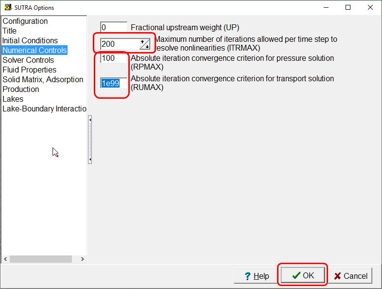
On the Numerical Controls tab, set ITRMAX to 200, RPMAX to 100, and RUMAX to 1E99.

Make no changes on the remaining tabs. Click OK to save your changes.

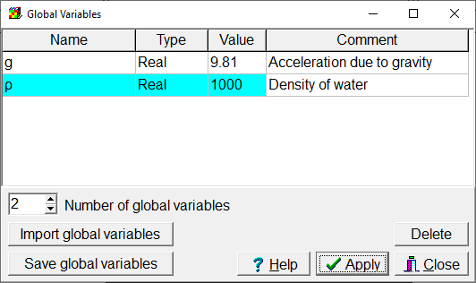
The model has a specified pressure boundary on the left side. The pressure increases with depth. We will define two global variables that we will use in a formula for the specified pressure "g" is the acceleration due to gravity and "ρ" is the density of water. Select "Data|Edit Global variables" and set g to 9.81 and ρ to 1000. Then click the Apply button. (If ρ does not appear on your keyboard, you can copy it from this document and paste it the dialog box using Ctrl-C and Ctrl-V.)

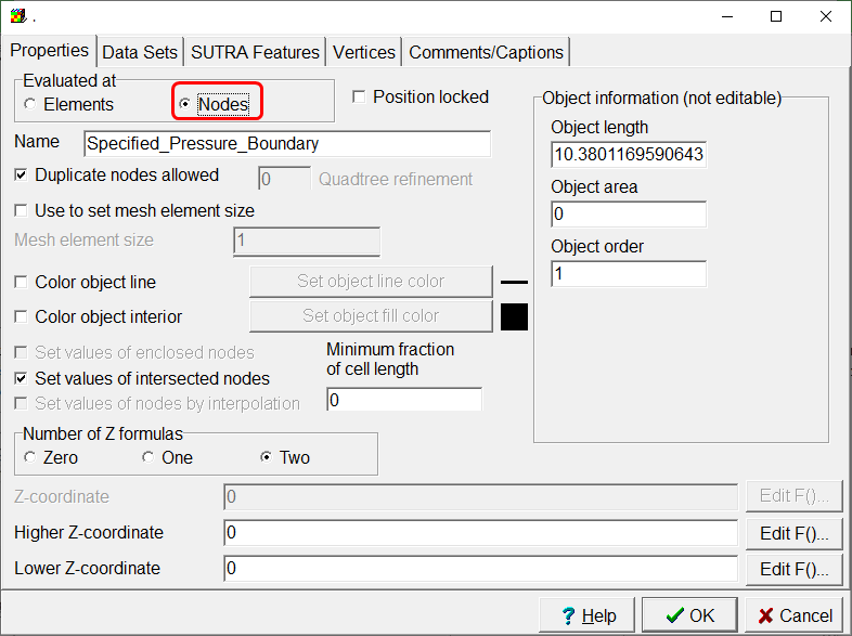
To create the specified pressure boundary, click the create straight line button and draw an object just inside the left edge of the model. On the Properties tab, set Evaluated At to Nodes.

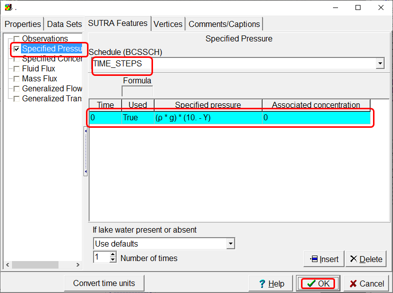
The pressure along the boundary will be ρg*Depth. ModelMuse can calculate the depth as "10-Y" so the formula for specified pressure will be (ρ * g) * (10. - Y).

You can color the grid with the specified pressure to make sure it is being calculated properly. The pressure should be 0 in the top node and 98,100 in the bottom node.

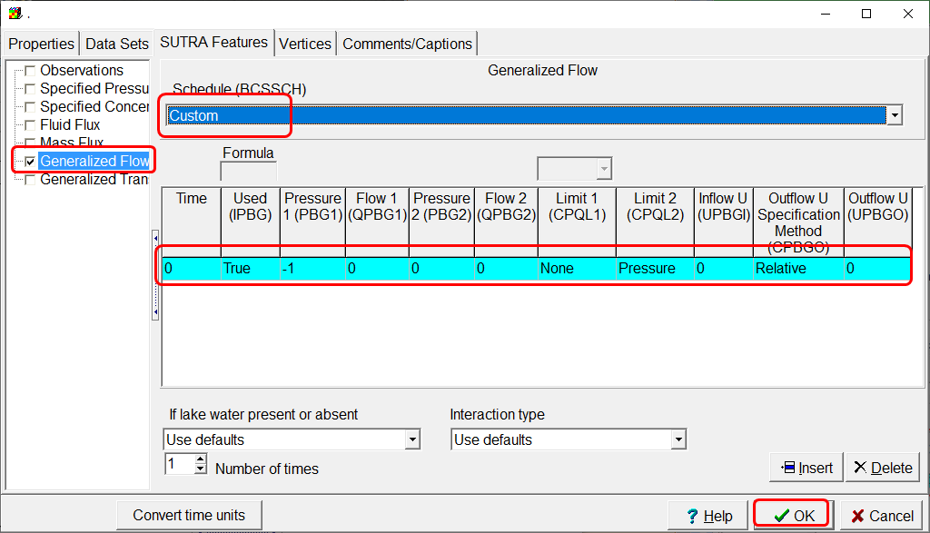
The generalized-flow boundary is along the right edge of the mesh. So draw another object just inside the right edge of the mesh. As with the specified pressure boundary, set "Evaluated At" to "Nodes."  Set the properties of the Generalized Flow Boundary as illustrated below and click OK.

Time = 0

Used = True;

Pressure 1 = -1

Flow 1 = 0

Pressure 2 = 0

Flow 2 = 0

Limit 1 = None

Limit 2 = Pressure

Inflow U = 0

Output U Specification Method = Relative

Outflow U = 0

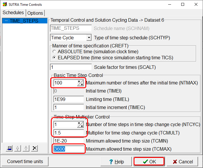
Select Model|SUTRA Time Controls and change the following values.

NTMAX = 100

NTCYC = 1

TCMULT = 1.5

TCMAX = 3600

Then click OK.

Select Model|SUTRA Output Control and change NPRINT to 10 on the Listing File tab and NCOLPR and LCOLPR to 10 on the Nod and Ele Files tab.

The aquifer properties are all uniform. Specify the following properties in the Data|Edit Data Sets dialog box.

You are now ready to run the model by selecting "File|Export|SUTRA Input Files." You will get a warning about using the Direct solver but you can ignore it.

When the model has finished running, you can import the model results by selecting "File|Import|Model Results..." Here we are importing all the data types except Concentration for the final time step and contouring the pressure.

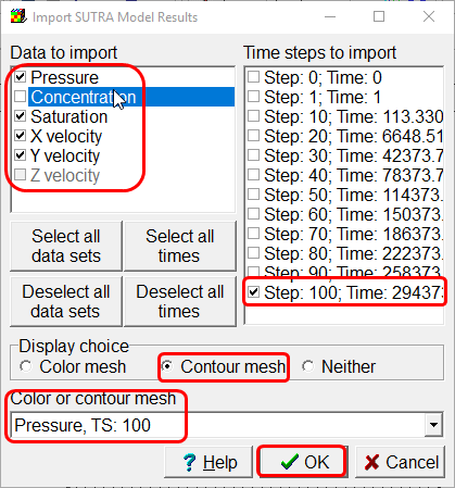
You can adjust the contour interval and display flow vectors using the Data|Data Visualization dialog box.