Lake Example

This example approximately reproduces the example from page 35 of the SUTRA 3.0 documentation. It uses the lake capability. Please read that section to better understand this example. We will start by creating a steady-state SUTRA model without lakes to determine the initial conditions. Then we will add lakes all over the top surface of the model.

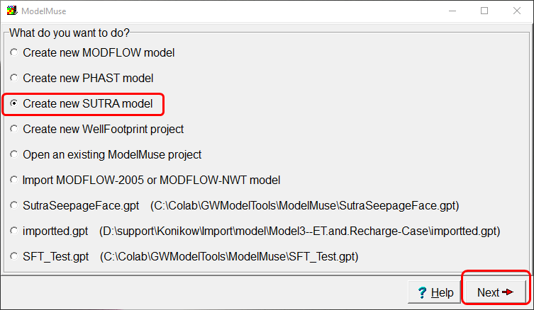
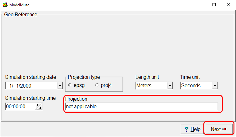
Start by creating a new SUTRA model. Because this is a hypothetical model, the projection of the model doesn't apply.

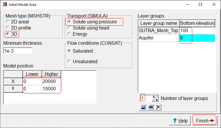
Set the model as a 3D model using using pressure. The model will end up being 20,000 meters long, 10,000 m wide and 100 m high so set the lower position of X and Y to 0 and the higher positions to 20,000 and 10,000 respectively and the thickness of the single aquifer to 100. (The aquifer will be divided vertically later.) Then click the "Finish" button.

We will use the Fishnet Mesh option to define the mesh. The size of the elements will be 500 x 500 so there will be 40 elements in the X direction and 20 elements in the Y direction.

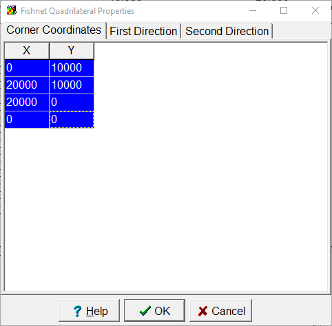
Click the Draw fishnet mesh quadrilaterals button and click in the main window to outline an area approximately 20,000 m long by 10,000 meters wide. When you are done, double click inside the quadrilateral and set the four corners of the quadrilateral to (0, 10,000), (20,000,10,000), (20,000,0), and (0,0).

Set the Discretization in the first and second directions so that there will be 40 elements in the X direction and 20 in the Y direction.

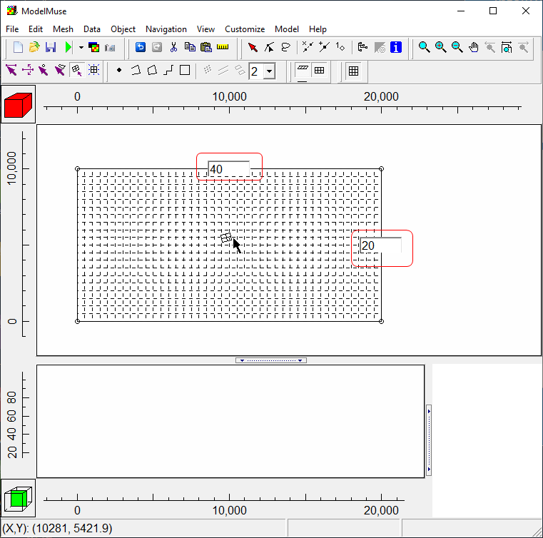
Click the Generate Mesh button and then click the OK button to generate the mesh.

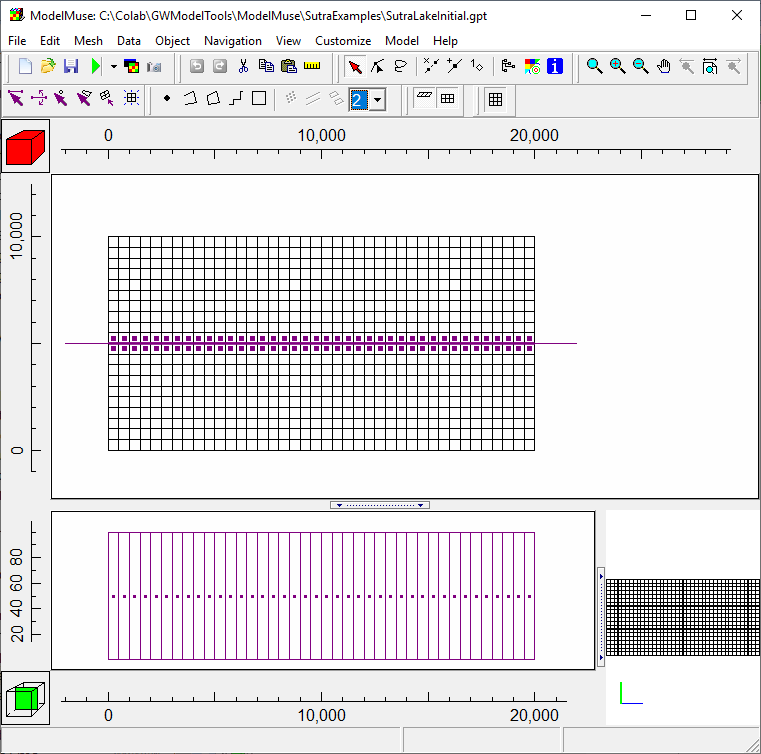
The top of the model will be defined with the following equation.

where r3, r4, and r5 are defined by the following equations.

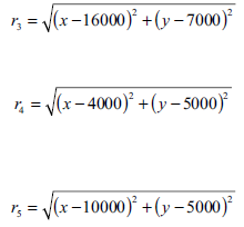
In ModelMuse, we can create data sets for  r3, r4, and r5 and assign values to them using formulas.  Select "Data|Edit Data Sets" and add new Data Sets names R3, R4, and R5. Each data set should be a 2D data set that is evaluated at nodes. Use the following formulas.

Be sure that all three data set are evaluated at notdes. Then select the SUTRA_Mesh_Top data set and specify it with the following formula.

((100. - (15. / (1. + Power((R3 / 1500.), 4.)))) - (20. / (1. + Power((R4 / 2000.), 4.)))) - (30. / (1. + Power((R5 / 3000.), 4.)))

 

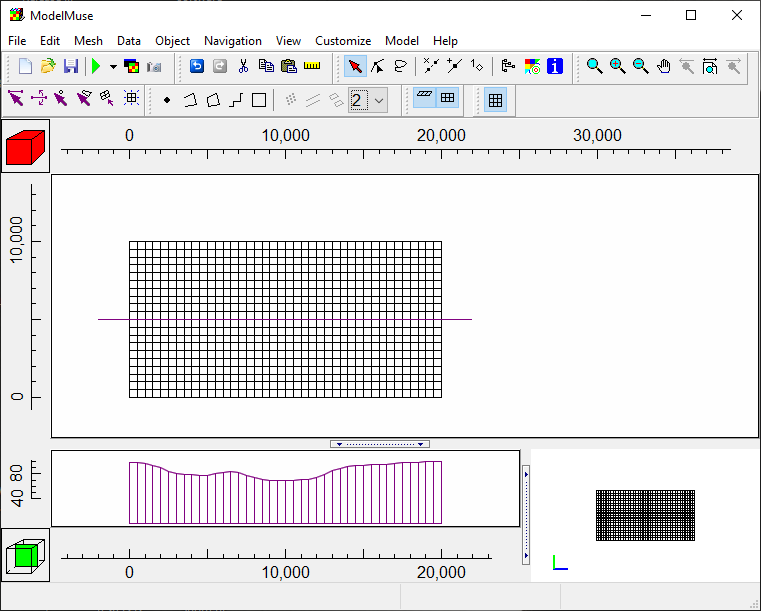
The model should be discretized into 10 elements vertically. To do that select Model|SUTRA Layer Groups and set the vertical discretization to 10.

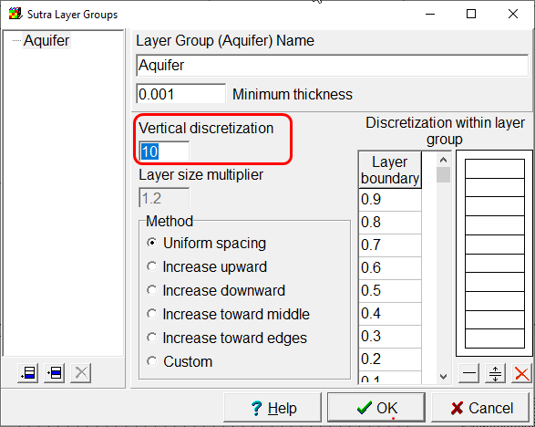
Next, select Data|Edit Data Sets and change the default formulas for the following data sets.

Next, select Model|SUTRA Options and set the following values.

Next select Model|SUTRA Time Controls and set the following values. (The initial time increment, TIMEC is equivalent to 1 week.)

Select Model|SUTRA Output Control and set NPRINT to 100. Uncheck CPANDS, CVEL, and CCORT. On the Node and Ele Files pane, set NOCLPR, LCOLPR to 100. On the Obs and Boundary Conditions Files pane, set all the values to 100 except NLAKPR; set it to 10.

The model has a specified pressure of 0 over the entire upper surface. Create an object that covers the top of the model. The object should be evaluated at nodes and have a single Z formula. The Z formula should be SUTRA_Mesh_Top. On the SUTRA Features tab, define a specified pressure boundary with a pressure of zero.

Save the ModelMuse file and run the model (File|Export|SUTRA Input Files).

We will use the simulated pressures from this model to specify the initial pressures in the model with lakes. Select "File|Import|Model Results." Select the .nod file for the model and import the pressure in time step 0. If desired, you can also import the velocities from time step 1.

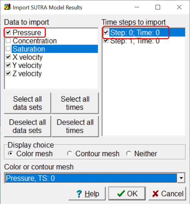
If you imported the velocities, you can use the Data|Data Visualization dialog box to color the mesh and display flow vectors.

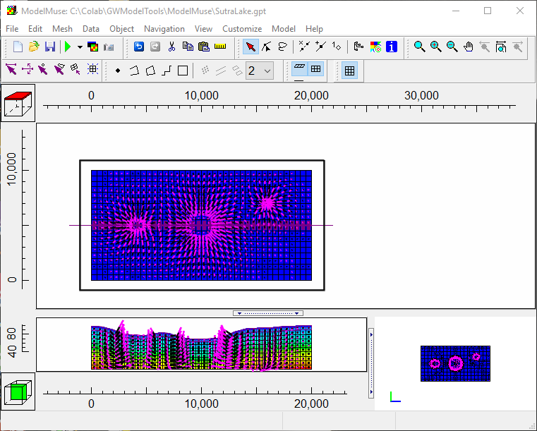
Now would be a good time to save your model. Then save it with a different name. The new model will be converted to a transient model with lakes. Initially the lakes are dry but that will change. All the nodes on the top surface will be eligible to form lakes.

We will use the simulated pressures from the steady-state model as the initial heads in the transient model.Select "Data|Edit Data Sets" and rename the "Pressure_0" data set under "Optional|Model Results|Pressure" to "PInitial." When you click the Apply button, the data set will be renamed and will now be classified under "User Defined" instead of "Optional." Now change the formula for the "InitialPressure" data set to "PInitial."

Select Model|SUTRA Options and make the following changes.

In the modified model, the specified pressure boundary has an associated concentration that changes from 0 to 1 after 30 weeks in a block of nodes in the upper right corner. We will create a new data set to define the concentration associated with the specified pressure and then use that in the formula in the specified pressure boundary.

Select "Data|Edit Data Sets." Create a new data set named concentration that is evaluated at nodes.

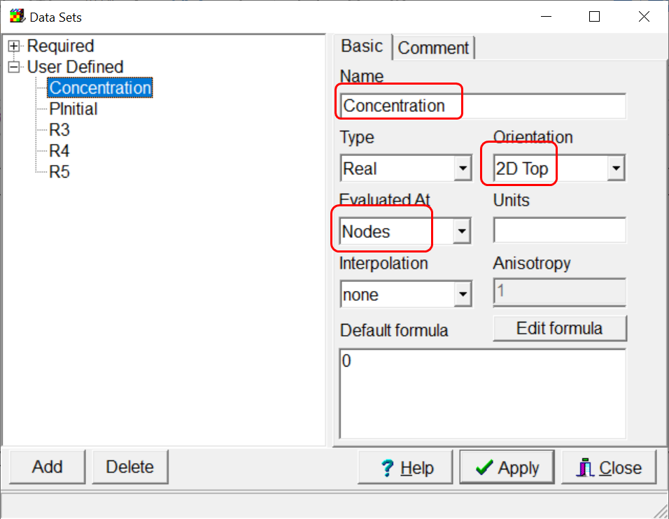
Next, create an object in the upper right corner of the model that encompasses a block of 6 x 6 nodes. Set "Evaluated At" to nodes and have it set the Concentration data set to 1. The number of Z formulas doesn't matter.

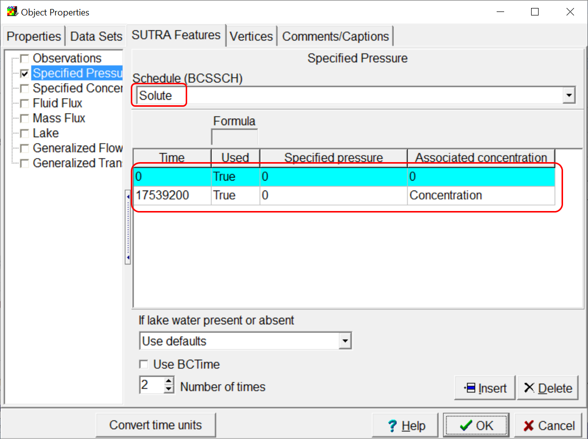
Next, we define a new time schedule that we will use with the specified pressure boundary. Select SUTRA Model|Time Controls and add a new time schedule with the following characteristics.

Then edit the object that defines the specified pressure boundary. Set the schedule to Solute and for the second time set the associated concentration formula to the Concentration data set.

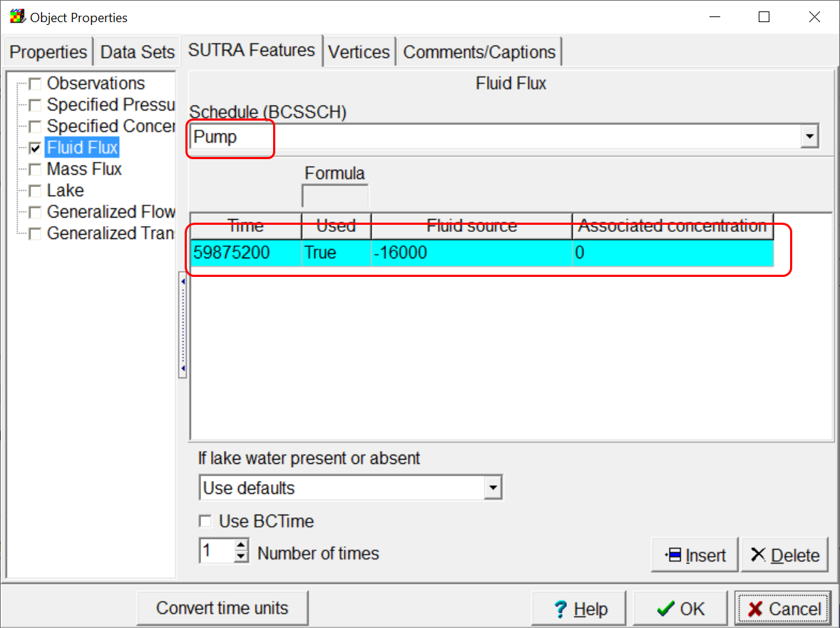
The model has a well at the center of the middle lake in the very center of the model. It will start pumping at 100 weeks. We will define a schedule for it with the following characteristics

Create a point object in the center of the model. Set Evaluated At to nodes and set the Number of Z formulas to 1. Set the Z formula to SUTRA_Mesh_Top. On the SUTRA Features tab, specify a fluid flux boundary using the Pump schedule and setting the fluid source to -16000.

Now run the model again.

We will create an animation of the lakes over time.

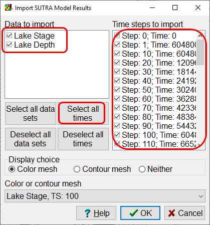
Select File|Import|Model Results and select the .lkst file. The Import SUTRA Model Results dialog box will appear. Click the Select all times button so that all the data sets and times are selected. Then click the OK button to import the data.

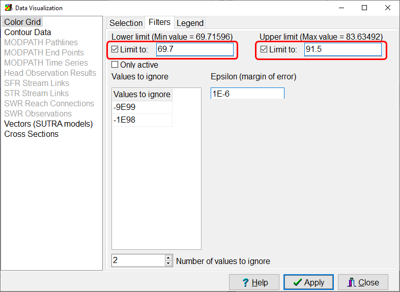
The highest lake stage of 91.498 will be at time step 100. the lowest stage of 69.716 will be at time step 1. Use the Data|Data Visualization dialog box to color the grid with the lake stage at time step 1. On the Filters tab, check the check boxes for the lower and upper limits and enter values of 69.7 and 91.5.  

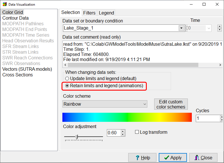
Next, go back to the Selection tab and select Retain limits and legend (animations). this will ensure that in the animation, the colors for the data set will maintain consistent values.

Next, select File|Export|Image. On the View pane on the left, uncheck all the check boxes. On the Text pane, enter the following two lines for the title

Time Step = %TS

Elapsed Time = %ET

Note that the two macros, %TS and %ET are set to the time step and elapsed time for the data set as specified in the data set comment.

On the Animation pane, check the checkbox for Lake Stage and then uncheck the checkbox for Lake_Stage_0.

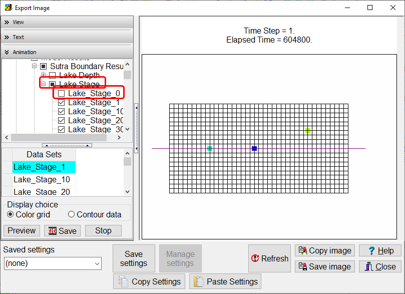
Click the Preview button to view the animation of the lake stage. Note how the lakes grow, merge, and then separate again.