PEST Examples

The examples presented here are variations of the Rocky Mountain Arsenal example included in the help in previous versions of ModelMuse. The previous tutorial showed how to simulate this conceptual model with MODFLOW-2005. For users unfamiliar with ModelMuse, it would be best to go through one or more of the previous examples to gain familiarity with ModelMuse. Instructions for the examples can be found under “Help|Examples.” Here, we will start with working MODFLOW 6, MODFLOW-2005, and SUTRA versions of the model and show how to use PEST with them. ModelMuse is distributed with three ModelMuse files for each version of the model. One of the files is used as the starting point of the exercise. Another model is a modified version of the first with spatially varying hydraulic conductivity and a different infiltration rate in a discharge pond. This was treated as the “true” model and was used to generate simulated values to use in the exercise. The final file contains the completed model after it has been set up to perform parameter estimation. For the MODFLOW-2005 simulation, there is a fourth file containing an imported version of the model following parameter estimation. The installer places these files in the sub folders of the “C:\Users\Public\Documents\ModelMuse Examples\examples\PEST” folder. If ModelMuse is installed manually, the files are in the “examples\PEST” folder of the distribution file.

The goal of these exercises is to learn how to specify observations and use parameters for both data sets and boundary conditions in ModelMuse and to learn how to visualize the characteristics of the calibrated model.

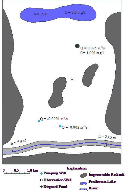
Before explaining how to use PEST with these examples, the conceptual model will be reviewed. The aquifer is simulated as confined. The steady-state model has a lake at the northern end and a stream at the southern end both of which are modeled as specified head boundaries as illustrated below. The lake has a head of 75 m. The stream head varies from 23.5 m near its eastern end to 5 m near its western end. Bedrock outcrops on the east, west, and south sides are considered impermeable and partially delimit the active area of the model. In addition, two bedrock outcrops within the model area are treated as inactive areas. A disposal pond in the northern half of the study area acts as a source of water and solute in addition to the lake. There are two production wells in the southern half of the model. The disposal pond is a potential source of contaminants to the production wells. The model is intended to help assess this problem. In the uncalibrated version of the model the flow rate out of the disposal pond is estimated at 0.03 m3/s. The estimated hydraulic conductivity is 0.0001 m/s. The models all have head observations and a flow observation. The head observations are scattered throughout the model area. The flow observation encompasses part of the discharge into the stream. The parameters to be estimated are the hydraulic conductivity and the flow rate of the disposal pond.

Because this model has only confined layers and the only boundary conditions are specified heads and specified flows, it is a linear model. That should make estimating parameters for this model easier than would often be the case in practice.