Using Formulas to Define Aquifer Properties

21.Only the portion of the aquifer within the domain outline and above the bottom of the lower aquifer should be active. The first step in making the correct elements active is to make the default formula for the Active data set “False” for all of the elements. To do this select Data|Edit Data Sets… and change the formula for the Active data set from “True” to “False.”

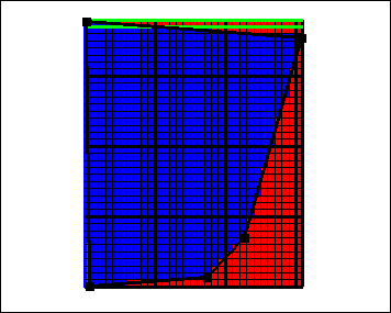
22.After clicking Apply to make the change in the Data Sets dialog box, double click on the “Domain_Outline” object. In the Object Properties dialog box, check Set values of enclosed elements, and change Higher Z-Coordinate to 9 and Lower Z-Coordinate to -271. On the Data Sets tab, check the checkbox for Active data set (under "Required|Hydrology"). Click button labeled Edit F()... above the Formula box for the Active data set to display the Formula Editor. Change the formula to “Z > Lower_Aquifer_Bottom.” (Z is found under Functions|GIS and Lower_Aquifer_Bottom is found under Data Sets.) This formula will evaluate to True for all elements whose centers are above the bottom of the lower aquifer. Click OK to close the Formula Editor and OK again to close the Object Properties dialog box. To check whether the Active data set is being set properly, select Data|Data Visualization|Color Grid…, select the Active data set (under " Sets|Required|Hydrology"), and click Apply. Click on the Selection cube for the top view of the model to change the selected layer and see the values of the Active data set in each layer (fig. 62). To view the Active data set in the 3-D view, it is convenient to show only the elements in which Active is true. To do so, select Data|Data Visualization|Color Grid… again, set the Lower limit to “True” and click OK. Only the elements for which the Active data set is true will be colored.

Figure 62. Active data set in the top layer of the Biscayne Bay aquifer model.

23.The next step is to define the hydraulic conductivity of the upper aquifer. This can be calculated from the data that have been imported by dividing the transmissivity by the saturated thickness. The saturated thickness is just the imported initial water table minus the bottom of the upper aquifer. To make this calculation, select Data|Edit Data Sets… Select the default formula for the "Upper_Aquifer_Kx" data set and click the Edit Formula button to display the Formula Editor. Set the formula to

Upper_Aquifer_Transmissivity / (Imported_Water_Table - Upper_Aquifer_Bottom)

and click OK to close the Formula Editor but leave the Data Sets dialog box open.

24.The next step is to use this hydraulic conductivity to help set the distribution of the Kx data set used by PHAST. Select the default formula for the Kx data set and display the Formula Editor. Set to formula to

If(Z > Upper_Aquifer_Bottom, Upper_Aquifer_Kx, 20)

(This formula assigns a value of 20 to the hydraulic conductivity of the lower aquifer.) If can be found under Functions|Logical. Z can be found under Functions|GIS. “Upper_Aquifer_Bottom” and “Upper_Aquifer_Kx” can be found under Data Sets. Click OK to close the Formula Editor and click Apply to make the changes in the Data Sets dialog box. Try coloring the grid by the Kx data set. (It may take a few seconds for the screen to be refreshed because Kx needs to be calculated.)

25.The hydraulic conductivity in the Y direction (Ky) will be set to the hydraulic conductivity in the X direction. The hydraulic conductivity in the Z direction (Kz) will be set to the hydraulic conductivity in the X direction divided by 10. To set these values, select Data|Edit Data Sets… Select the default formula for the Ky data set. Set its formula to “Kx”. Select the default formula for the Kz data set. Set its formula to “Kx / 10.”. Click Apply to make the changes in the Data Sets dialog box.