This shows how to reproduce the second example from the SUTRA 4.0 documentation where a more complete description of the model can be found. In it, an unsaturated profile model with 100 elements in the vertical direction and one element in the X direction is subjected to freezing and thawing. The model has two parts. In the first part, freezing occurs from the top down. In the second part, thawing occurs from the bottom up due to upward groundwater flow.
Part A Freezing Conditions
Generating the Mesh
Start the ModelMuse and select a 2D profile model in which Freezing transport and unsaturated flow are selected. The model will be two meters tall and one meter wide so select the model area to encompass the a rectangle extending from (0,0) to (1,2). Select Mesh|Draw Fishnet Mesh Quadrilaaterals and draw a quadrilateral covering the model area. You can type in exact coordinates after finishing drawing the fishnet mesh quadrilateral. When done specify 100 elements in the vertical direction and 1 element in the X direction. Then select Mesh|Genarate Mesh to generate the SUTRA mesh.
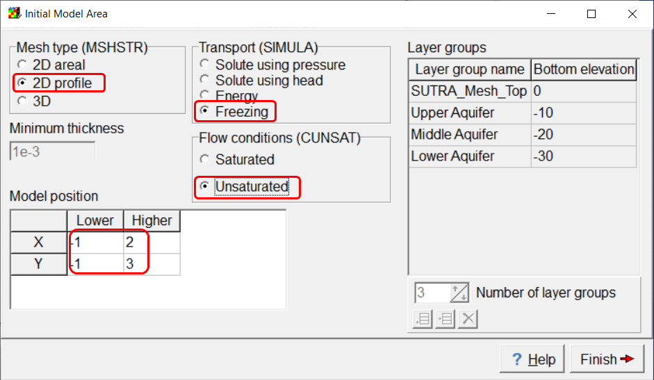
Screen capture of ModelMuse showing the model specifications
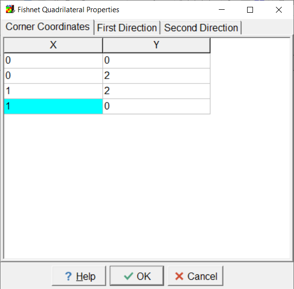
Screen capture showing to corner coordinates of the fishnet mesh quadrilateral.
SUTRA Options
Several changes need to be made in the SUTRA Options dialog box. Select Model|SUTRA Options.
•On the Configuration pane, select Transient flow, transient transport.
•On the Title pane, specify SUTRA 4.0 - Unsaturated Freeze/Thaw Example - Part A, Freezing of unsaturated unfrozen column starting at top.
•On the Numerical Controls pane, set TRMAX to 10, RPMAX to 275, and RUMAX to 999999.
•On the Fluid Properties pane, set DRLDU to 0.
•On the Total Water Saturation tab of the Region 1 pane, set SWMOD to Piecewise linear, SWRES to 0.01, and PSWRES to -20,000.
•On the Relative Permeability Parameters tab of the Region 1 pane, set RKMOD to Piecewise linear.
•On the Liquid Water Saturation tab of the Region 1 pane, set SLMOD to Piecewise linear.
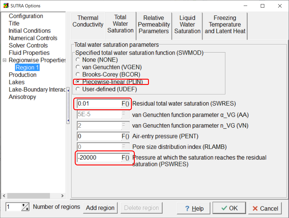
Screen capture of the Total Water Saturation tab for Region 1 with selected choices highlighted.
Time Schedules
Two time schedules are used for the model. Select Model|SUTRA Time Controls. For the TIME_STEPS schedule, set NTMAX to 99,999,TIMEL to 15,552,000, TIMEC to 8640, NTCYC to 99,99,999 TCMIN to 8.64E-16, and TCMAX to 172800.
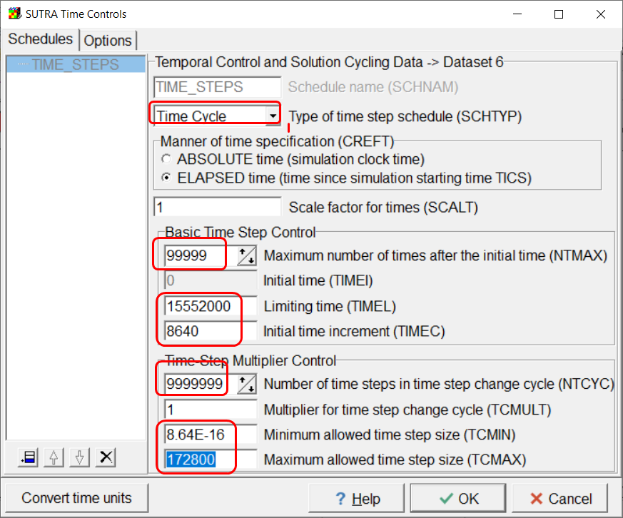
Screen capture of the SUTRA Time Controls dialog box illustrating the specification of the TIME_STEPS schedule.
Click the Add time schedule button to add a new time schedule. Set the Schedule name to Timed_Obs. Set SCHTYP to Step Cycle. Set both NSMAX and ISTEPL to 4500.Set ISTEPC to 10.
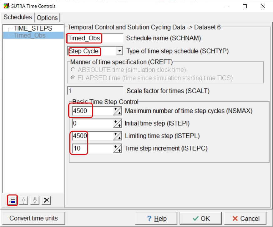
Screen capture of the SUTRA Time Controls dialog box showing the specificatin of the Time_Obs schedule.
SUTRA Output Control
Select Model|SUTRA Output Control. On the Listing File pane, set NPRINT to 10. On the Nod and Ele Files pane, NCOLPR and LCOLPR to 10 and check the check boxes for liquid saturation and ice saturation.
Aquifer Properties
Initially, the column is fully unsaturated with a pressure of 0 at the bottom and -19,620 at the top. This can be specified with the default formula of Interpolate(Y, 0., 0., -19620., 2.) for the InitialPressure data set. The initial temperature is 2. The longitudinal dispersivity is 0.01. The maximum permeability is 5E-12. The porosity is 0.3. The transverse dispersivity is 0.01. The default formulas for the other data sets can be left unchanged.
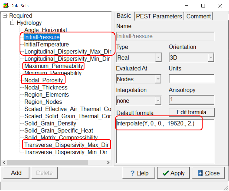
Screen capture of the Data Sets dialog box highlighting the data sets whose formulas need to be edited and the formula for the InitialPressure data set.
Boundary Conditions
All the boundary conditions use TIME_STEPS as their schedule. At the bottom of the column there are specified pressure, temperature, and fluid flux boundaries. Use a straight-line object drawn through the mesh at the lowest nodes to specify them. The specified pressure is 0 with an associated temperature of 2. The specified temperature is also 2. The fluid flux rate is 0 with an associated temperature of 2. (The Fluid flux boundary will be set to a non-zero value in the second part of the exercise.Use another straight-line object to define a specified temperature boundary and generalized flow boundary at the top of the mesh. The specified temperature is -8. For the generalized flow boundary, set Pressure 1 and Flow 1 to 0 Set Pressure 2 to 196.2. Set Flow 2 to -0.000496. Set Limit 1 to Flow. Inflow U is arbitrary. Set CUPBGO to Relative and Outflow U to 0.
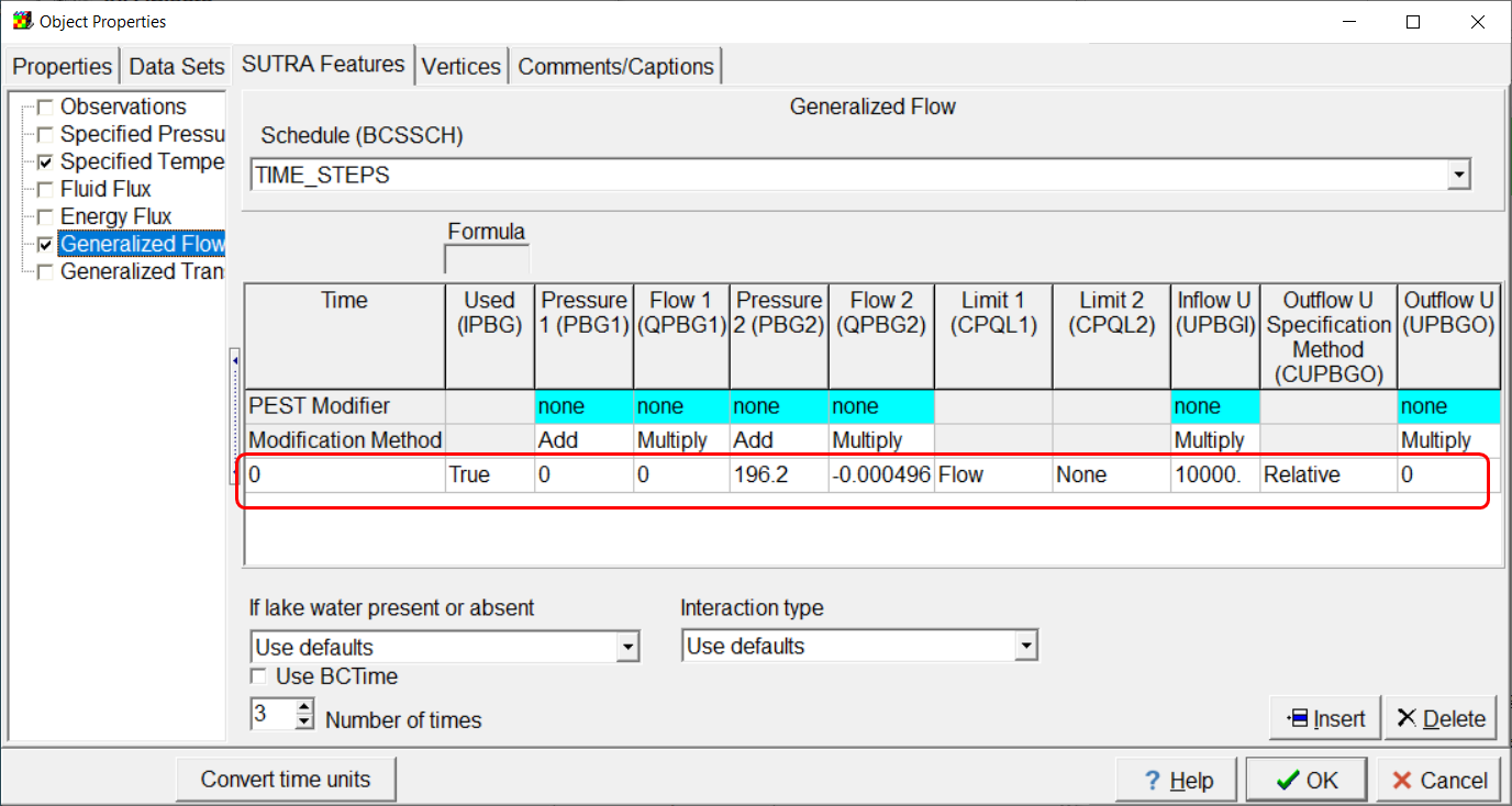
Screen capture of Object Properties dialog box showing the specification of a generalized flow boundary.
Observations
The entire left column of the model will be used for observations to enable plotting of graphs of aquifer properties. Use Timed_Obs as the time schedule. Set the observation format to OBC.
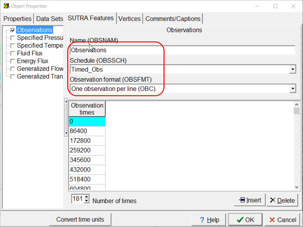
Screen capture of the Object Properties dialog box showing specification of observation times.
Run the Model
Export the SUTRA input files and run the model. The restart file from this model will be used to specify the starting conditions for the second part of the model in which thawing conditions are simulated.
Part B Thawing Conditions
Save your model with a new name for part B of this exercise in which thawing is simulated.
SUTRA Options
Many of the SUTRA options will remain the same but a few are changed.
On the Title pane, change the title to "SUTRA 4.0 - Unsaturated Freeze/Thaw Example - Part B (continued from Part A), Thawing of unsaturated partially frozen column due to water inflow at bottom"
On the Initial Conditions pane, choose to use the restart file for both the initial pressure and temperature and then select the restart file from part A
On the Production pane, check the check box to simulate production.
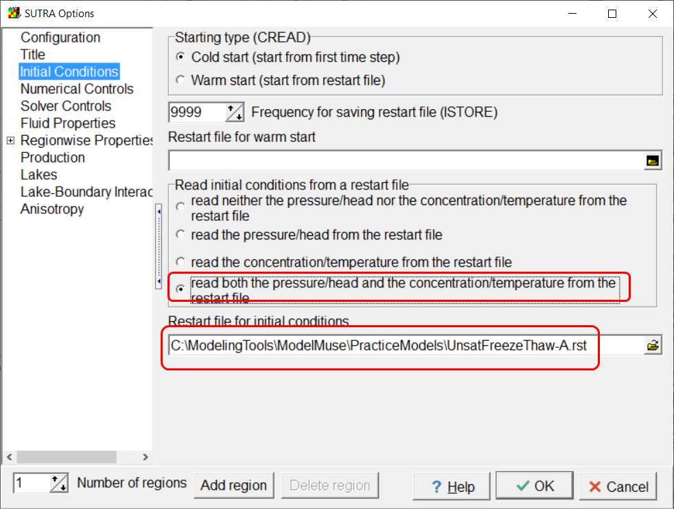
Screen capture of the SUTRA Options dialog box showing that the restart file is used for the initial conditions.
Time Schedules
In the SUTRA Time Controls dialog box for the TIME_STEPS schedule, change NTMAX to 999,999, TIMEC to 864, and NTCYC to 9,999,999. For the Timed_Obs schedule, change NSMAX to 18001, ISTEPL to 45,000, and ISSTEPC to 100.
SUTRA Output Control
In the SUTRA Output Control dialog box, change NPRINT to 100 and NCOLPR and LCOLPR to 100. For the observation and boundary condition files, increase all the values except NOBLIN from 9999 tp 99999
Boundary Conditions
For the bottom boundary, deactivate the specified pressure boundary, Change the starting time of the specified temperature and fluid flux boundaries to 864. Change the fluid flux rate to 5.787037037E-5. For the top boundary, deactivate the fluid flux boundary.
Model Results
After running the model, you can import the simulated values to obtain figures similar to those in the SUTRA 4.0 documentation. The data in the observation output files (.obc) files can be imported into spreadsheets and plotted to produce graphs similar to those in the SUTRA 4.0 documentation.