This shows how to reproduce the first example from the SUTRA 4.0 documentation where a more complete description of the model can be found. In it, a 4m x 4m contaminated zone is surrounded on two sides by a frozen wall and on a third size by the edge of the model in order to isolate the contaminated zone. The model is simulated with a 2D areal model. The following table shows the model properties and how those properties are implemented in ModelMuse
Parameter |
Implementation in ModelMuse |
Name |
Value and Unit |
aquifer thickness |
Data set |
Nodal_Thickness |
1 m |
model extent (east-west x, north-south y) |
|
|
25 m, 15 m |
porosity |
Data set |
Nodal_Porosity |
0.1 |
fluid compressibility |
Option/Fluid Properties |
COMPL |
4.47×10⁻¹⁰ [kg/(m s2)]-1 |
fluid specific heat |
Option/Fluid Properties |
CL |
4,182. J/(kg °C) |
fluid thermal conductivity |
Option/Fluid Properties |
SIGMAL |
0.6 J/(s m °C) |
linear fluid density function: [here set to a constant density of 1000. kg/m3] base density (RHOL0) base temperature (URHOL0) coefficient of density change (DRLDU) |
Option/Fluid Properties |
RHOL0 URHOL0 DRLDU |
1,000 kg/m3 20 °C 0 kg/( m3 °C) |
solid matrix compressibility (COMPMA) |
Data set |
Solid_Matrix_Compressibility |
1×10⁻⁸ [kg/(m s2)]-1 |
solid grain density (RHOS) |
Data set |
Solid_Grain_Density |
2,600 kg/m3 |
solid grain specific heat |
Data set |
Solid_Grain_Specific_Heat |
840 J/(kg °C) |
solid grain thermal conductivity |
Data set |
Scaled_Solid_Grain_Thermal_Conductivity |
3.5 J/(s m °C) |
ice compressibility (COMPI) |
Option/Fluid Properties |
COMPI |
0 [kg/(m s2)]-1 |
ice density |
Option/Fluid Properties |
Ice density (RHOI0) |
920 kg/m3 |
ice thermal conductivity |
Option/Fluid Properties |
SIGMAI |
2.14 J/(s m °C) |
ice specific heat |
Option/Fluid Properties |
CI |
2,108 J/(kg °C) |
latent heat of fusion |
Option/Regionwise Properties/Freezing Temperature and Latent Heat |
HTLAT |
3.34×10⁵ J/kg |
permeability (max and min) |
Data set |
Maximum_Permeability and Minimum_Permeability |
1×10⁻¹⁰ m2 (hydraulic conductivity ~10-3 m/s) |
longitudinal dispersivity (in max and min permeability directions) |
Data set |
Longitudinal_Dispersivity_Max_Dir and Longitudinal_Dispersivity_Min_Dir |
0.1 m |
transverse dispersivity (in max and min permeability directions) |
Data set |
Transverse_Dispersivity_Max_Dir and Longitudinal_Dispersivity_Min_Dir |
0.01 m |
gravity vector components (GRAVX, GRAVY) |
Option/Configuration |
GRAVX, GRAVY |
0, 0 m/s2 |
piecewise-linear liquid-water saturation function: minimum liquid saturation (SLSATRES) temperature at which minimum liquid saturation occurs (TLRES) |
Option/Regionwise Properties/Liquid Water Saturation |
SLMOD SLSATRES TLRES |
0.01 –2 °C |
piecewise-linear relative permeability function: liquid saturation at which minimum relative permeability occurs (SLRKMIN) minimum relative permeability (RKMIN) |
Option/Regionwise Properties/Relative Permeability Parameters |
RKMOD SLRKMIN RKMIN |
0.01 1×10⁻⁶ |
|
|
|
|
Numerical parameters/controls |
|||
finite elements (in x,y directions) -fishnet mesh- |
|
|
100, 60 |
initial time step |
SUTRA Time Controls/Schedules |
TIMEC |
1 hr = 3600 sec |
time step change cycle (NTCYC) |
SUTRA Time Controls/Schedules |
NTCYC |
1 |
time step multiplier (TCMULT) |
SUTRA Time Controls/Schedules |
TCMULT |
1.02 |
maximum allowed time step (TCMAX) |
SUTRA Time Controls/Schedules |
TCMAX |
730.5 hr (= 1 month) = 2629800 sec |
time steps in pressure and temperature solution cycle (NPCYC, NUCYC) |
SUTRA Time Controls/Options |
NPCYC, NUCYC |
1, 1 |
maximum time steps in simulation (NTMAX) |
SUTRA Time Controls/Schedules |
NTMAX |
1,000 (any number ≥ 420) |
maximum absolute simulation time |
SUTRA Time Controls/Schedules |
TIMEL |
1×10⁵ hr = 360,000,000 sec |
|
|
|
|
output cycles (NPRINT, NCOLPR, LCOLPR) |
SUTRA Output Control |
NPRINT, NCOLPR, LCOLPR |
10, 10, 10 |
iterations for nonlinearity (ITRMAX) |
Options/Numerical Controls |
ITRMAX |
1 |
solver for pressure, solver for temperature |
Options/Solver Controls |
CSOLVP, CSOLVU |
DIRECT, DIRECT |
observation locations (5 selected nodes along southern edge, y = 0 m, figure 5) |
|
|
x = 90 m, 130 m, 170 m, 210 m, 250 m |
observation output cycle NOBCYC |
no longer part of the input |
|
1 |
|
|
|
|
Initial and boundary conditions |
|||
initial temperature of aquifer |
Data set |
InitialTemperature |
+5 °C |
temperature of cooling system |
Object/SUTRA Features |
Specified Temperature |
specified T = -5. °C |
initial pressure of aquifer |
Data set |
InitialPressure |
p = 500 – 20x [kg/(m s2)] |
initial temperature of column |
|
|
+2 °C |
west boundary condition for fluid mass balance |
Object/SUTRA Features |
Specified Pressure |
specified p = 500 [kg/(m s2)] (~5 cm hydraulic head) -- inflowing water has T = +5 °C |
east boundary condition for fluid mass balance |
Object/SUTRA Features |
Specified Pressure |
specified p = 0 [kg/(m s2)] (0. cm hydraulic head) -- any inflowing water has T = +9,999 °C (none ever flows in here) |
east and west boundary conditions for energy balance |
|
|
insulated (energy enters via the western inflow and exits via the eastern outflow) |
Generating the Mesh
Start model and select a 2D areal model with Freezing Transport. Select the model area to encompass the area where the mesh will be located.

Screen capture of the ModelMuse Initial Model Area dialog box with 2D areal and Freezing transport selected.
The mesh is 25 m long in the X direction and 15 m wide in the Y direction. The mesh elements are square and the distance between nodes is 0.25 m. To create the mesh, select Mesh|Draw Fishnet Mesh Quadrilaterals and draw a quadrilateral over the mesh area. In the Fishnet Mesh Quadrilaterals dialog box, set the coordinates to cover the correct area. Set the discretization to 60 in the Y direction and to 100 in the X direction. Select Mesh|Generate Mesh to create the mesh.

Screen capture of the Fishnet Quadrilateral Properties dialog box showin the quadrilateral corner coordinates

Screen Capture of ModelMuse showing the discretization in the X and Y directions.
SUTRA Options
There are a number of changes that need to be made in the SUTRA Options dialog box.
•On the Configuration pane, select Transient flow/transient transport.
•On the Title pane, enter "SUTRA 4.0 - Saturated Groundwater Freezing Example, Containment by Frozen Groundwater Wall."
•On the Fluid Properties pane, set DRLDU to 0.

Screen capture of the Fluid Properties pane showing the value of DRLDU.
•On the Production pane check the check box to simulate production.
One Region is predefined in the Regionwise properties. More could be added if desired. For this model, only one region needs to be defined. Five tabs are present on the Region 1 pane. Changes need to be made on two of those panes: Relative Permeability Parameters and Liquid Water Saturation.
•On the Relative Permeability Parameters tab, select Piecewise linear and set RKMIN to 1E-6 and SLRKMIN to 0.01.

Screen capture of the Relative Permeability Parameters tab illustrating changes to be made on this tab.
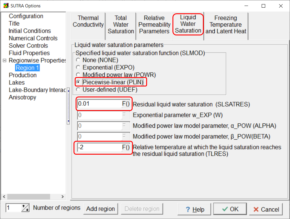
On the Liquid Water Saturation tab, select Piecewise-linear and set SLSATRES to 0.01 and TLRES to -2.
Time Schedules
The model uses two time schedules. One is the TIME_STEPS schedule required for all SUTRA models. The other is used with the observations. For the TIME_STEPS schedule, set NTMAX to 1000, TIMEL to 360,000,000, TIMEC to 3600, NTCYC to 1, TCMULT to 1.02, TCMIN to 3600, and TCMAX to 2,629,800. The second schedule is named Timed_Obs. Set SCHTYP to Step Cycle, NSMAX to 2100, ISTEPI to 0, ISTEPLto 2100, and ISTEPC to 1.

Screen capture illustrating the values assigned to the TIME_STEPS schedule.

Screen capture illustrating the values assigned to the Timed_Obs schedule.
Output Control
In the Model|SUTRA Output Control dialog box, set NPRINT to 10 and NCOLPR and LCOLPR to 10. For the Node and Element files, print liquid saturation and ice saturation.

Screen capture of the ModelMuse SUTRA Output Control dialog box showing some items that should be specified in the model.
Contaminated Zone
In this example, the contaminated zone is represented by a fluid flux boundary with a flux rate of zero. The temperature of the associated flux can be set to any value. The zone should encompass all the nodes for (11,4), through (15,0). Because the flux rate is zero, the boundary does not affect the model results. However, you could set the flux rate to a positive value to see how that would affect the model results. A positive flux rate could represent recharge.
Specified Pressures
Specified pressures of 0 and 500 are present on the East and West edges of the model respectively. Use straight-line objects to define them. The specified pressure boundary on the West side of the model should have an associated temperature of 5 °C. The associated temperature of the Eastern boundary can be any value.
Specified Temperature
The specified temperature boundary is in an L-shaped region upstream (West) and to the North of the contaminated zone with a temperature of -5 °C. One node separates the specified temperature boundary from the contaminated zone.

Screen capture of ModelMuse showing the specified temperature boundary colored green.
Observations
Five observation locations are defined. They are located at (5,0), (13,0), (17,0), (21,0), and (25,0). If desired, you can use the node number at the observation location in the observation name. Use the Timed_Obs" sAll the observation formats should be Multiple observations per line (OBS).
Initial Conditions
The InitialPressure and InitialTemperature data sets define the initial conditions for the model. The initial temperature is a uniform 5 °C. The initial pressure varies linearly from 500 at the West end to 0 at the East end. Both can be specified using default formulas in the Data|Edit Data Sets dialog box. One suitable formula for the initial pressure is "Interpolate(X, 500., 0., 0., 25.)".
Aquifer Properties
The aquifer is assumed to be isotropic and the data sets that define properties in the "minimum" direction are linked to the data sets in the "maximum" direction so that all that needs to be done is set the default properties in the "maximum" direction.
Data Set |
Formula |
Longitudinal_Dispersivity_Max_Dir |
0.1 |
Maximum_Permeability |
1e-10 |
Nodal_Porosity |
0.1 |
Nodal_Thickness |
1 |
Transverse_Dispersivity_Max_Dir |
0.01 |
Model Results
After running the model, you can plot the ice saturation and groundwater velocity vectors by importing data from the .nod and .ele files.

Screen capture of the Import SUTRA Model Results dialog box illustrating the import of the ice saturation and x and y velocities.

Plot of Ice Saturation and Velocity Vectors at Time Step 40.
The data from the .obs file or files can be imported into a spreadsheet program and plotted.