RmaSutra: Visualize Modified Model Input

The model created by PEST after parameter estimation now has a different flow rate through the disposal pond and non-uniform maximum and minimum hydraulic conductivity distributions. ModelMuse provides ways to import both sets of data and visualize both.

Visualizing Specified Flow Rates

Select File|Import|SUTRA Features. Then select the either the SUTRA.FIL file or the RmaSutra.inp file. In the dialog box, select the time step for which to see the pumping rates. In this case select time step 0. ModelMuse will create a data set named SP_Flow_TS_0 with flow rate at each node. The data set will be classified under "Optional|Model Results|Model Features." You can color the grid with this data set. The sum of the flow rates for the specified flow that  are part of the disposal pond is 0.012. The true value is 0.025. This new data set does not change how the pumping rate is defined in ModelMuse so if you export the model input files from ModelMuse again, it will use the original pumping rates defined in ModelMuse not the ones that PEST generated.

Visualizing Maximum and Minimum Hydraulic Conductivity

There are two ways to import the new hydraulic conductivity data sets. One way is to select File|Import|Gridded Data Files and select the file for the hydraulic conductivity data sets in the arrays subdirectory of your model directory. The new data sets will be classified under "User Defined|Created from text file." The names of the new data set will be based on the names of the files. Another method to import the data is to select File|Import|SUTRA Files and select the .15B file. The new data sets will be classified under "Optional|Model Results|Model Features|Imported from SUTRA data set 15B file." ModelMuse will import all the elementwise data from this file.

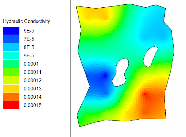
A diagram of the estimated distribution of  hydraulic conductivity is shown below.

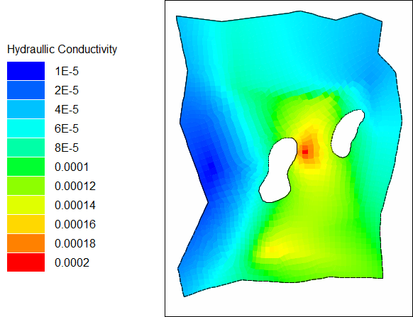
The true distribution from the model used to generate the observed values for the parameter estimation exercise is shown below.

Both the estimated and true hydraulic conductivity distributions show patches of low hydraulic conductivity on the west and north east portions of the model with a higher hydraulic conductivity between the two bedrock islands. The true distribution has more extreme high and low values.