RmaSutra: Tikhonov Regularization |
RmaSutra: Tikhonov Regularization |
By default, ModelMuse will define several regularization equations for you. Including such equations allows the user to inform the level of fit as well as helps stabilize the parameter estimation process. Tikhonov regularization information is defined on the Prior Information Group Properties, Initial Value Prior Information, Within-Layer Continuity Prior Information, and Between-Layer Continuity Prior Information panes on the PEST Properties dialog box.
When PEST performs parameter estimation in regularization mode, each parameter is compared with a preferred value. The first type of regularization equation compares the current value of the parameter to its preferred value as represented by the initial value specified by the modeler at the beginning of parameter estimation. This preferred condition is applicable to all parameters. A second type, a preferred homogeneity condition, only applies to parameters that are associated with pilot points. With those, the current value of a pilot point value is compared with the values of neighboring pilot points applied to the same zone. The third type of regularization equation also only applies to parameters that are associated with pilot points, but the preferred homogeneity condition is evaluated at the same parameter at the same location on adjacent layers. Finally, the degree of fit the modeler desires is specified by the PEST PHIMLIM variable (Fienen and others, 2009; Doherty and Hunt, 2010; Anderson and others, 2015, Chapter 9). PHIMLIM represents a target measurement objective function, which controls the tradeoff between fit and adherence to preferred parameter conditions. Typically, for the first run of PEST PHIMLIM is set very low (10-10) to discard the parameter preference and assess the best fit possible for a given conceptual model; then that best-fit objective function is increased (for example, 110% of the best fit value), specified as the new PHIMLIM value, and PEST re-run. Typically, PHIMACCEPT will be changed to be 5-10% larger than PHIMLIM. The reader is directed to Fienen and others (2009) and Chapter 9 in Anderson and others (2015) for additional discussion of this critically important PEST variable.
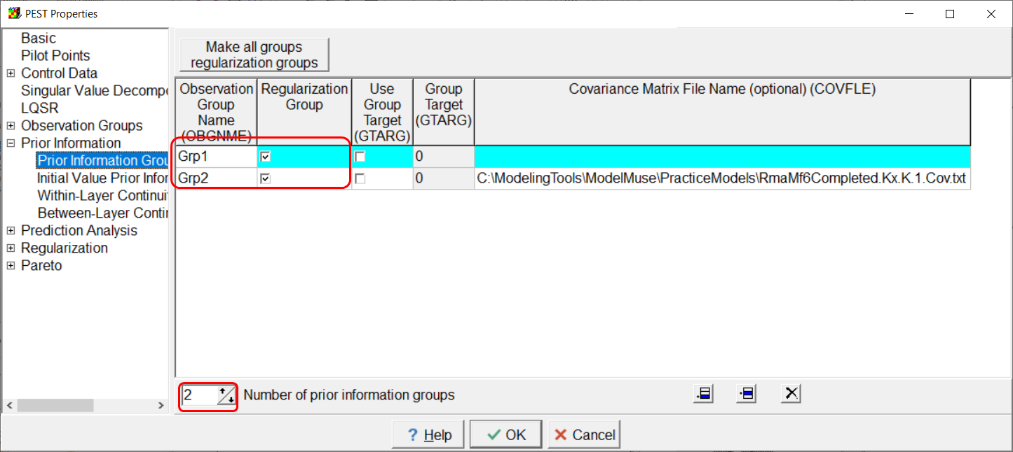
Open the PEST Properties dialog box and go to the Prior Information Group Properties pane. Define two groups and make them regularization groups as illustrated below.

Screen capture of the PEST Properties dialog box after creating a new prior information group.
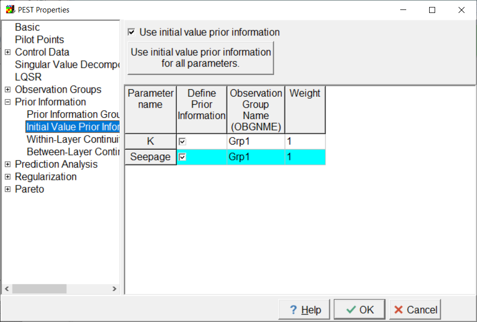
On the Initial Value Prior Information pane assign both parameters to one of the groups as illustrated below.

Screen capture of the PEST Properties dialog box showing the assignment of parameters to a prior information group.
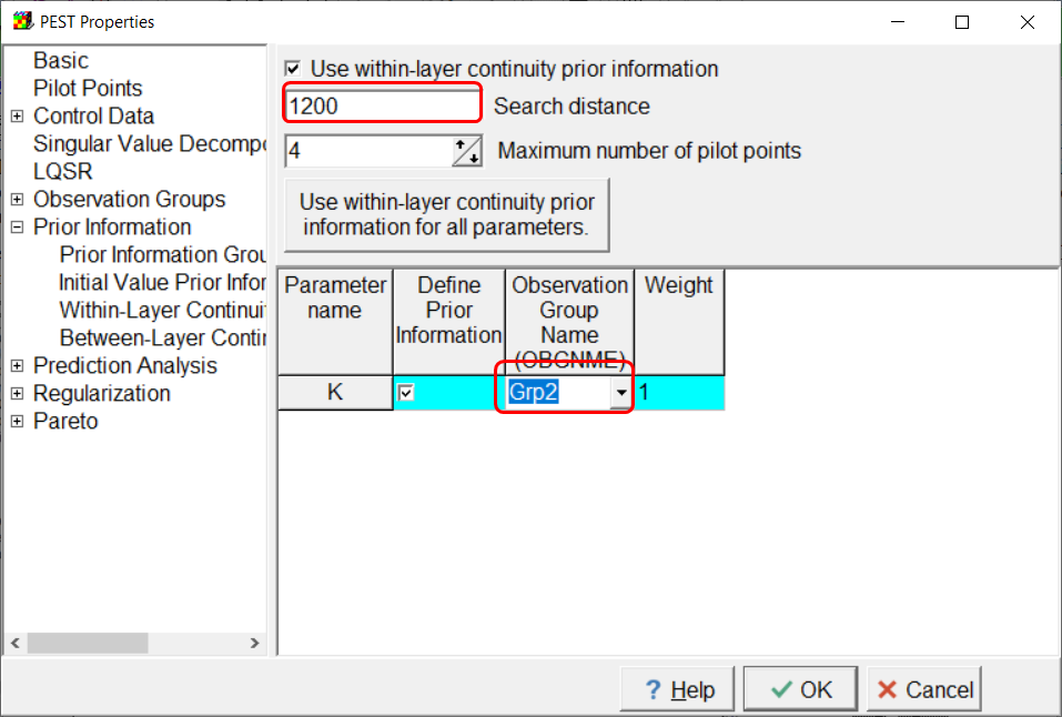
Next go to the Within-Layer Continuity Prior Information pane and specify the search distance and the observation group name as illustrated below.

Screen capture of the Within-Layer Continuity Prior Information pane showing the definition of prior information.
We do not need to deal with the between-layer prior information because the model only has one layer.