Rivers

8.This model has three rivers: the Little River, the North Fork River and the North Canadian River. The Little River is defined by a polyline object with vertices at (44000., 15000.), (44000., 0.), and (90000., 0.). Draw a polyline object on the top view of the model at approximately those locations. (When drawing the object, it is possible to see the current location of the cursor in the status bar.) In the Object Properties dialog box, select the Nodes radio button. Change the Name of the object to “Little_River.” Check the Set values of intersected nodes checkbox. Then go to the Vertices tab and correct the locations of the vertices to be exactly correct.

9.On the PHAST Boundary Conditions tab, select a River boundary, and set the following properties.

 

 

In the table for the river boundary set the Associated solution to 1. The head must vary along the length of the river. A formula can be used to accomplish this. Click on the cell in the table for head and observe the F() button that appears. Click it. This will open the Formula Editor. Click the Help button and read about this dialog box.

9.The head in Little River should vary from 335 at the upstream end to 275 at the downstream end. The Interpolate or MultiInterpolate functions can be used to achieve this goal. On the right side of the Formula Editor, click on the “+” next to Functions to display the types of functions that are available. Then click on the “+” next to Math to display all the math functions. Click on MultiInterpolate in this list. Then click the Function Help button. The help system will open and display help on the MultiInterpolate function. Read the description of the MultiInterpolate function to learn what it does. Go back to the Formula Editor and double-click on MultiInterpolate. Note that MultiInterpolate appears in the Formula text box along with its parameters. Go back to the List of Data Sets and Functions and click on the “-” next to Math and then click on the “+” next to Object. Select FractionOfObjectLength and click on the Function Help button again. Read the description of what FractionOfObjectLength does. FractionOfObjectLength will be used as the first parameter in MultiInterpolate in the Formula text box of the Formula Editor. Select “Position” in the Formula text box and double-click on FractionOfObjectLength. Next substitute 335 and 275 for “Value1” and “Value2” respectively. Substitute 0 and 1 for “Distance1” and “Distance2” respectively. Remove the extra square brackets and dots so that the final formula is “MultiInterpolate(FractionOfObjectLength, 335., 0., 275., 1.).” Click OK to close the Formula Editor and then click OK again to close the Object Properties dialog box.

10.The North Fork River is entered in the model in a similar fashion. The coordinates of its vertices are (30000, 36000), (30000, 48000), and (90000, 48000). Its Hydraulic Conductivity, Width, Depth, Bed Thickness, and Associated Solution are all the same as in the Little River. The heads at the upstream and downstream ends are 335 and 280 respectively so the formula for head is “MultiInterpolate(FractionOfObjectLength, 335., 0., 280., 1.).”

11.The North Canadian River is entered in the model in a similar fashion. The coordinates of its vertices are (60000, 30000), and (90000, 20000). Its Hydraulic Conductivity, Width, Depth, Bed Thickness, and Associated Solution are all the same as in the Little River. The heads at the upstream and downstream ends are 350 and 305 respectively so the formula for head is “MultiInterpolate(FractionOfObjectLength, 350., 0., 305., 1.).”

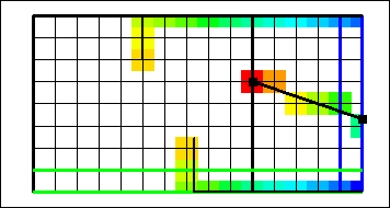
12.Make the selected layer the bottom layer and then try coloring the grid (Data|Data Visualization|Color Grid…) with the River_Head (under Boundary Conditions|PHAST River) (fig. 54).

 

Figure 54. The top view of the model with grid cells colored to reflect the river head in example 3. The river objects are shown with red lines.