Henry 2D Model

The simulation of the Henry (1964) problem is described in the SUTRA documentation (Voss and Provost, 2002). It consists of a vertical box 2 m long and 1 m high with freshwater inflow on the left side and a saltwater boundary on the right. The mesh consists of square elements that are 0.1 m on a side. This model illustrates how to use a steady-state simulation to provide the initial pressures for a transient simulation. In the steady-state model, there is a specified pressure boundary on the right with a concentration of 0 and inflow of freshwater from the left. In the transient model, the specified pressure boundary is changed to have a concentration equal to that of seawater. The system is then allowed to evolve until it reaches a nearly steady-state condition. This example also illustrates how to check that boundaries have been set up as intended and how to animate the results of a simulation.

Simulation for initial conditions.

1.Start ModelMuse and select Create new SUTRA model. Click the Next button. Specify "Not Applicable" for the projection. Then click the Next button again.

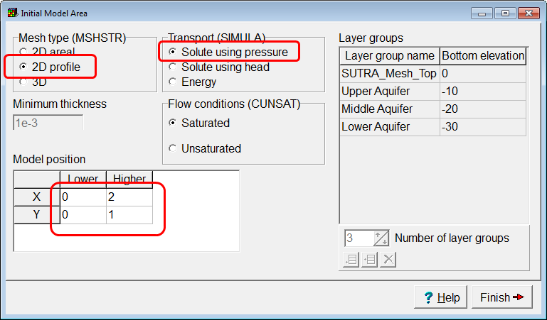
2.Set the Mesh type to 2D profile, Transport to Solute using pressure and for Model position, set the lower value for both coordinates to 0, the higher X coordinate to 2 and the higher Y coordinate to 1. Then click the Finish button.

3.Select View|Vertical Exaggeration and the set the vertical exaggeration to 1.

4.The next step is to create the mesh. Because we want a perfectly regular mesh, we will use the "fishnet mesh" approach. Select Mesh|Draw Fishnet-Mesh Quadrilaterals or click on the Draw fishnet-mesh quadrilaterals button.

5.To draw the quadrilateral click four times in the main window to draw a quadrilateral. Try to click at approximately the following coordinates: (0,0), (2,0), (2,1), and (0,1). You don't need to be exact. We'll set the coordinates exactly in a later step.

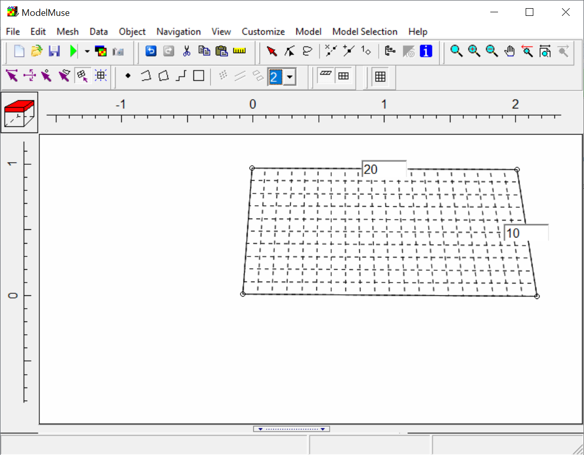
6.After you click on the fourth coordinate, the fishnet quadrilateral will be created. Control will appear on two sides of the quadrilateral. Enter values of 20 and 10 in the two controls so that 20 elements will be created along the horizontal edge and 10 elements will be created along the vertical edge.

7.Now double-click in the center of the fishnet-mesh quadrilateral. The Fishnet Quadrilateral Properties dialog box will appear. The First Direction and Second Direction tabs in this dialog box are used to specify how the elements are distributed along the side of the quadrilateral. By default, they are uniformly distributed which is what we want so we won't be doing anything on those tabs. Switch to the Corner Coordinates tab and enter the precise coordinates we want for the corners of the quadrilateral. Those are (0,0), (2,0), (2,1), and (0,1). Then click OK.

8.Now select Mesh|Generate Mesh... or click the Generate mesh button. The Mesh Generation Method should already be set to Fishnet and the renumbering method does not apply in this case. Just click the OK button and the mesh will be generated.

9.Select Navigation|Restore Default 2D View or click the Restore default 2D view button to center the mesh in the ModelMuse main window with an appropriate magnification.

10.The next step is to create a fluid source along the left edge of the model. Select Object|Create|Straight Line or click the Create straight line object button and then create an object near the left edge of the mesh stretching from the top to the bottom of the mesh. In the Object Properties dialog box, change Evaluated at to Nodes. Switch to the Sutra Features tab and check the check box for Fluid Flux on the left. Change the Number of times to 1. In the table, there should be 1 row. In the Time column set the time to 0. Check the checkbox in the Used column. In the Fluid source column set the formula to "(0.066 * ObjectIntersectLength) / ObjectLength" and in the Associated concentration set the formula to 0.

11.The formula for the fluid source is intended to provide a total source of 0.066 divided among the nodes on the left edge of the model. However, for the fomula to work properly, we need the object to reach exactly from the top to the bottom of the mesh. To do that go to the Vertices tab and change one of the Y coordinates to 1 and the other one to 0. Then click OK.

12.To make sure the fluid source was applied correctly, we will color the grid with the fluid source value. Select Data|Data Visualization or click the Data visualization button. Select Color Grid on the left and for Data set or boundary condition, select Fluid Flux. Set the Time to 0 and click Apply. You should end up with something like this.

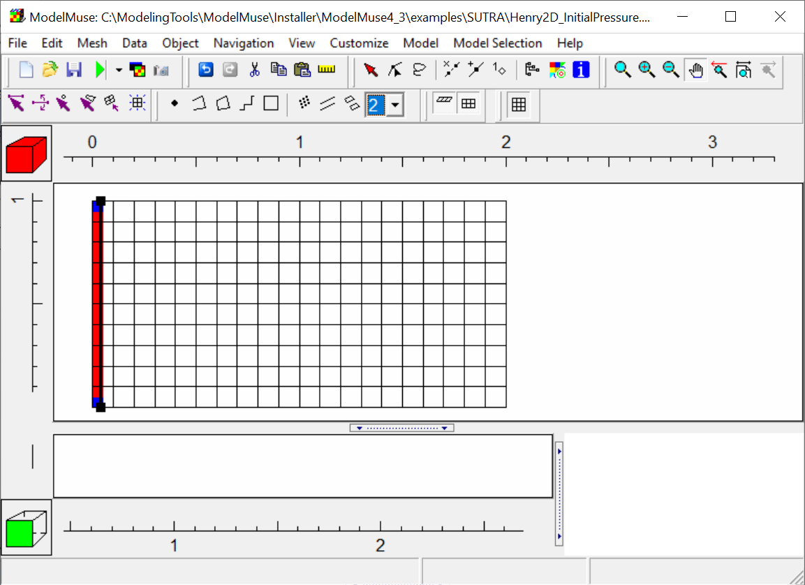
13.If you place the cursor over one of the colored cells, the value applied to the node will be displayed in the third panel on the status bar. For the red cells, the value should be 0.066. For the blue cells, it should be 0.033.

14.The next step will be to define the specified pressure on the right side of the mesh. We will use the following formula for the density of water as a function of concentration (1000. + 700. * Concentration). We will specify the concentration as 0.0357 and we will also need to specify a value for gravity (9.8). We will use global variables to specify the seawater concentration and gravity. Select Data|Edit Global Variables... and define two global variables named SeaWaterConcentration and Gravity. They should both be real numbers with values of 0.0357 and 9.8 respectively.

15.Now we will create the specified pressure boundary. Select Object|Create|Straight Line or click the Create straight line object button and then create an object near the right edge of the mesh stretching from the top to the bottom of the mesh. In the Object Properties dialog box, change Evaluated at to Nodes. Switch to the Sutra Features tab and check the check box for Specified Pressure or the left. Change the Number of times to 1. In the table, there should be 1 row. In the Time column set the time to 0. Check the checkbox in the Used column. In the Specified pressure column set the formula to "((1000. + (700. * SeaWaterConcentration)) * Gravity) * (1. - Y)" and in the Associated concentration set the formula to 0.

16.To make sure the specified pressure was applied correctly, we will color the grid with the specified pressure. Select Data|Data Visualization or click the Data visualization button. Select Color Grid on the left and for Data set or boundary condition, select SUTRA Specified Pressure. Set the Time to 0 and click Apply. You should end up with something like this.

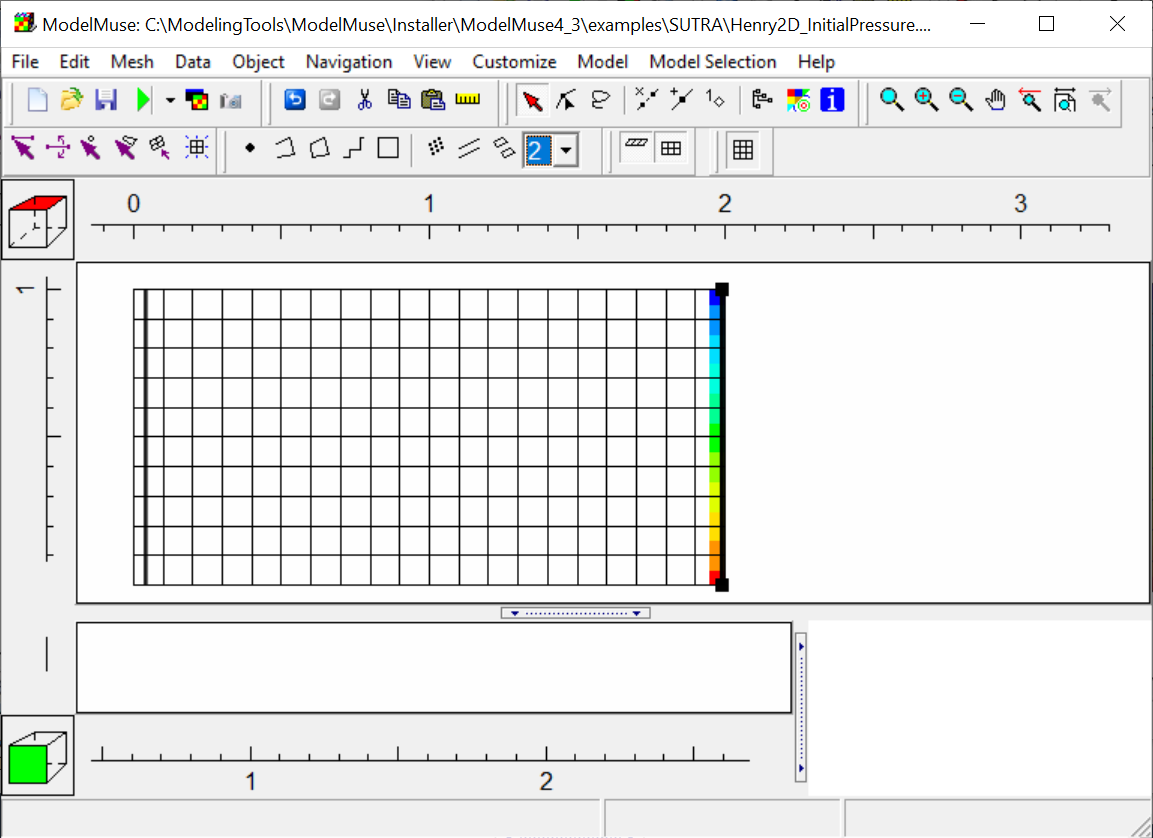
17.You can check the specified pressures in the same way you checked the fluid flux. The specified pressures should range from 10044.902 at the base to 0 at the top.

18.The final step for this model is to set a few of the aquifer properties. We will set the longitudinal and transverse dispersivities to 0, the permeability to 1.020408E-9, and the porosity to 0.35. Select Data|Edit Data Sets... and under Required|Hydrology, select each of the appropriate data sets and set the formulas to the correct values and click Apply.

19.We also need to set a few controls in the SUTRA Options dialog box before we will be ready to run the model. Select Model|SUTRA Options...

a)On Configuration pane, set GRAVY to -9.8.

b)On the Title pane, set the title to "Henry Problem from SUTRA Documentation: variable-density benchmark problem." The first two lines that you enter will be printed to the SUTRA output file.

c)On the Fluid Properties pane, set Fluid compressibility to 0 and Fluid diffusivity to 1.88571E-5.

d)Click OK.

20.Select File|Save and save the ModelMuse project as Henry2D_InitialPressure.gpt.

21.Select Mode|SUTRA Program Location and check to make sure that the location for SUTRA is correct.

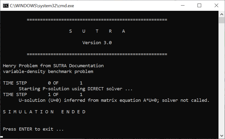
22.Now select File|Export|SUTRA Input files or click the Run SUTRA button. SUTRA will open in a command-line window and run. You can close the window when you are done. We will use the restart file from this model to define the initial pressures in the transient model.

Simulation for Transient Condtions

1.Save the previous model with a new name: Henry2D.gpt. We will modify this to be a transient model with seawater on the right boundary.

2.The first step is to change the model to a transient model. Select Model|SUTRA Options... On the Configuration pane, change the Simulation type to Transient flow, transient transport.

3.Switch to the Initial Conditions pane. For starting type, select cold start. Under Read initial conditions from restart file, select Read the pressure/head from restart file. Then select the restart file from the previous model (Henry2D_InitialPressure.rst). Click OK to close the dialog box.

4.Next, select Model|SUTRA Time Controls... For the TIME_STEPS schedule, change NTMAX from 1 to 100 and change TIMEC to 60.

5.We will also add another schedule that we will use with the observations we plan to set up later. Click the Add time schedule button. Then set the name of the new schedule to '"Timed_Obs." Change the type of schedule to a Step Cycle. Then set NSMAX and ISTEPL to 500 and click OK.

6.We also need to change when results are printed. Select Model|SUTRA Output Control... On the Listing File pane, change NPRINT to 50. Then on the NOD and ELE Files pane, change NCOLPR and LCOLPR to 10. Click OK to close the dialog box.

7.The next step is to the observation locations. We will have observations at the nodes on the bottom edge of the model between 1.0 and 1.9 on the X axis. Select Object|Create|Polygon or click the Create polygon object button. Create a polygon object that surrounds the desired nodes. In the Object Properties dialog box, change Evaluated At to nodes and switch to the SUTRA Features tab. Check the check box for Observations on the left. Select an arbitrary Name for the observations and set the Schedule to Timed_Obs. Click OK. Because this object is evaluated at nodes, the nodes that are enclosed by the object will be observation locations. To have an observation made at an arbitrary location, you could have used a point object.

8.When we set up the specified pressure boundary on the right, we set its concentration to 0. We need to change that to the concentration of seawater. Make sure you have the Select objects button depressed and double-click on the specified pressure boundary to open it in the Object Properties dialog box. Go to the SUTRA Features tab and set the formula for the associated concentration to "SeaWaterConcentration." Recall that SeaWaterConcentration is the name of a global variable that we set up earlier.

9.Next save and then run the model.as you did before.

10.This time we will take a look at the model results but first we will hide all the objects. Select Object|Show or Hide Objects... or click the Show or hide objects button. Uncheck the checkbox labeled All Objects.

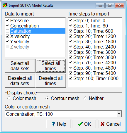
11.Next we will import the model results. Select File|Import|Model Results... or click the Import and display model results button. Select the Henry2D.nod file and click the Open button. The Import SUTRA Model Results dialog box will be displayed.

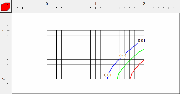
12.Uncheck Saturation because this is a fully saturated model. Select Contour Mesh and select the concentration for time step 100 as the data set to contour. Click the Select All Times button. Click the OK button to import the data.

13.You should now have contours similar to these.

14.Next we will animate the contours. To do that we first need to make sure that the values for the contour lines will be the same at each time step in the animation. Select Data|Data Visualization or click the Data visualization button. Select Contour Data on the left. Change the Contour interval to 0.005 and click the Apply button. Then check the Specify contours check box. If you wish, you can click the Edit contours button for more control on the contour values that will be used. Click the Apply button again.

15.Next click the Retain limits and legends (animations) radio button and click the Apply button again. Now set the data set to Concentration_0 and click the Apply button again. Click the Edit contours button to check that the contour values for Concentration_0 is the same as it was for Concentration_100. When the selected data set changes during the animation, the contour values for Concentration_0 will be applied to each succeeding data set.

16.Select File|Export|Image... or click the Export image button. On the Export Image dialog box, select the Text panel. In the title box type "Time Step = %TS; Time = %ET" The "%TS" and "%ET" are replaced with the time step number and the elapsed time in the title above the mesh image.

17.Now go to the Animation tab. Check the check box for "U values" under "Data Sets|Optional|Model Results." This will add all the concentration data sets to data sets table.

18.Set the Display choice to Contour data. Make sure you have resized the Export Image dialog box so that you can see the whole mesh and then click the Preview button. You should see the evolution of the concentration contours through time.