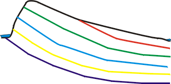
In many cases, a cross sectional model can be a good approach to a modeling problem. Because a cross sectional model will typically have far fewer cells than an equivalent three-dimensional model it can be run and calibrated much more quickly. Even if you will eventually need to use a three-dimensional model, starting with a two-dimensional model may provide you with insights into the system that will be helpful in three-dimensional modeling.
In this example, we will model the monocline illustrated below. The black line represents the ground surface. The colored lines are the boundaries between different geologic units and the blue areas on either end represent rivers. The uppermost geologic unit is missing for approximately half of the cross section and all but the bottom unit are missing at the far left. The rivers will be treated as constant-head boundaries. The right, and bottom boundaries are treated as no-flow boundaries. In the case of the boundary on the right, this might not be correct because the geologic units continue beyond the area shown on the cross section. However, flow observations in the rivers show that groundwater is discharging to the rivers and unless the geologic units provide a substantial barrier to flow, groundwater flow in the vicinity of the river is likely to be vertical. Vertical flow would be parallel to the edge of the model and would be a valid no-flow boundary for horizontal flow. Recharge enters the system at a rate of 10-9 m/s. The hydraulic conductivity varies between units but for simplicity they will all be treated as having hydraulic conductivities of 10-4 m/s except for the fourth unit (between the light blue and yellow lines) which has a hydraulic conductivity of 10-7 m/s. The cross section is 30,000 m long and surface elevations range from 50 m at the river on the right to 100 m at the top of the crest.
