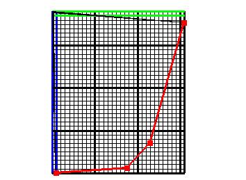
Two boundary conditions will be defined in this model: a specified head of zero on the eastern edge of the model (the ocean), and a specified flux of 4 inches per year through the top of the model (recharge).
26.To define the specified flux boundary, select Object|Create|Rectangle and draw a rectangle that completely encloses the top view of the model. ). In the Object Properties dialog box, change Evaluated At to Nodes, change the Name to “Specified_Flux”, check Set values of intersected nodes, change Number of Z formulas to One, and change Z-Coordinate to “9.” On the PHAST Boundary Conditions tab, select Flux boundary and change the Flux for time zero to -4. (The flux is negative because it is downward.) The associated solution does not need to be specified because this model does not simulate chemistry. Click OK to close the Object Properties dialog box.
27.To define the specified-head boundary, select Object|Create|Polyline and draw a polyline on the top view of the model on the eastern edge of the model (fig. 63). In the Object Properties dialog box, change Evaluated At to Nodes, change the Name to “Specified_Head”, and check Set values of intersected nodes. On the PHAST Boundary Conditions tab, select Specified head and change the Head for time zero to 0. Click OK to close the Object Properties dialog box. Try coloring the grid by the two boundary conditions (Specified_Head and Top_Flux_Boundary_Flux) to make sure they are applied properly.

Figure 63. Object representing a specified-head boundary (in red) in the Biscayne Bay aquifer model.