Data Set 0
|
[#Text]
Item 0 is optional -- “#” must be in column 1. Item 0 can be repeated multiple times.
Text - is a character variable (up to 199 characters) that starts in column 2. Any characters can be included in Text. The “#” character must be in column 1. Text is printed when the file is read.
|
|
Data Set 1
|
NPTH NLOC IOUTADV KTFLG KTREV ADVSTP FSNK [IMPATHOUT IMPATHOFF]
NPTH - is the total number of advective-transport paths that will be used (that is, the total number of repetitions of ITEM 3).
|
NLOC - is the total number of advective-transport observation locations that will be used (that is, the total number of repetitions ITEM 4).
|
IOUTADV – is a flag and a unit number.
| • | If IOUTADV > 0, it is the unit number to which the particle-tracking information will be written. |
| • | If IOUTADV = 0, particle-tracking information will not be written. |
|
KTFLG – is a flag indicating how the particle-tracking time step is calculated..
| • | If KTFLG = 1, particles are displaced from one cell face to the next, and the time-step length varies. |
| • | If KTFLG = 2, particles are displaced using the time steps specified by ADVSTP. |
| • | If KTFLG = 3, both of the above are included. |
|
KTREV – is a flag indicating the direction of particle displacement.
| • | If KTREV = 1, particles are displaced in a forward direction. |
| • | If KTREV = -1, particles are displaced in a backward direction. |
|
ADVSTP – is the particle-tracking time-step length to be used when KTFLG equals 2 or 3.
|
FSNK – is a flag and a fraction indicating how weak sinks are treated. Performs identically to Option 3 for terminating pathlines in MODPATH (Pollock, 1989, p. 34).
| • | If FSNK < 0, particles will be discharged at cells with any amount of discharge to boundary conditions. |
| • | If FSNK > 0, particles will be discharged at cells where discharge to sinks is larger than the specified fraction of the total inflow to the cell. |
|
IMPATHOUT – is a flag and a unit number.
| • | If IMPATHOUT > 0, it is the unit number to which particle tracking information will be written using the conventions of the MODPATH pathline file. |
| • | If IMPATHOUT = 0, no file is produced. |
|
IMPATHOFF – is a flag indicating the convention used to interpret the offsets in items 3 and 4 (see Anderman and Hill, 2001, p. 49). The offsets for particle starting locations are defined in input item 3 by variables SLOFF, SROFF, and SCOFF. The offsets for observation locations are defined in input item 4 by variables LOFF, ROFF, and COFF. If IMPATHOFF is omitted or set to zero, the offsets in the ADV2 input file need to be defined using the ADV2 convention. If IMPATHOFF equals 1, the offsets need to be defined using the MODPATH convention.
|
|
|
If porosity is to be defined using parameters, Item 2 must be entered as shown below and followed by Items 2a. and 2b.
The capability to define some porosity values using parameters and others without using parameters is not provided. Thus, if parameters are used to define the porosity, then they must define porosity for all model cells and Quasi-3D confining beds. Conversely, if porosity is defined using layer arrays, then no porosity parameters can be defined.
|
Data Set 2 (with parameters)
|
PARAMETER NPADV IPFLG
IPFLG – is the print code for all ADV parameters, which controls the printing of the porosity arrays created when the parameters are substituted into the arrays.
|
|
|
Repeat Items 2a-2b for each parameter to be defined (that is, NPADV times).
|
Data Set 2a
|
[PARNAM PARTYP Parval NCLU]
PARNAM – is the name of a parameter to be defined. This name can consist of up to 10 characters and is not case sensitive.
All parameter names must be unique.
|
PARTYP – is the type of parameter to be defined. For the ADV2 Package, the supported parameter types are:
| • | PRST – defines the effective porosity of the material represented by a model layer. |
| • | PRCB – defines the effective porosity of the material represented by a quasi-3D confining unit. |
|
NCLU – is the number of clusters required to define the parameter. Each repetition of item 2b is called a cluster, with variables Layer, Mltarr, Zonarr, and IZ.
|
|
|
Data Set 2b
|
[Layer Mltarr Zonarr IZ]
Each repetition of Item 2b is called a parameter cluster. Repeat Item 2b NCLU times.
Layer – is the model-layer number to which a cluster definition applies. Even if the Hydrogeologic-Unit Flow package (Anderman and Hill, 2001) is used, the effective porosity is defined by model layer, not hydrogeologic unit.
|
Mltarr – is the name of the multiplier array to be used to define array values that are associated with a parameter. The name “NONE” means that there is no multiplier array, and the array values will be set equal to Parval.
|
Zonarr – is the name of the zone array to be used to define array elements that are associated with a parameter. The name “ALL” means that there is no zone array and that all elements in the model layer are part of the parameter.
|
IZ – is up to 10 zone numbers (separated by spaces) that define the array elements that are associated with a parameter. These values are not used if Zonarr is specified as “ALL”. Values can be positive or negative, but 0 is not allowed. The first zero or non-numeric value terminates the list.
|
|
|
If porosity is not to be defined using parameters, Item 2 must be entered as shown
|
Data Set 2 (without parameters)
|
PRST(NCOL,NROW)
Item 2 is read using the array-reading utility module U2DREL (Harbaugh and others, 2000, p. 86-88. Item 2 is repeated for each model layer and quasi-3D confining unit in the grid. Thus, the number of PRST arrays must equal the number of model layers plus the number of quasi-3D confining beds. These layer variables are read in sequence going down from the top of the system.
PRST – is the porosity of the porous medium represented by a model layer or quasi-3D confining unit.
|
|
Items 3-4 are repeated as a group for each advective-transport path to be defined (that is, NPTH times).
|
Data Set 3
|
NPNT SLAY SROW SCOL SLOFF SROFF SCOFF
NPNT – is the number of observation points along the path being defined.
|
SLAY – is the layer of the initial location.
|
SROW – is the row of the initial location.
|
SCOL – is the column of the initial location.
|
SLOFF – is the layer offset used to locate the initial location within the finite-difference cell (must range between –0.5 at the bottom of the layer and 0.5 at the top of the layer).
|
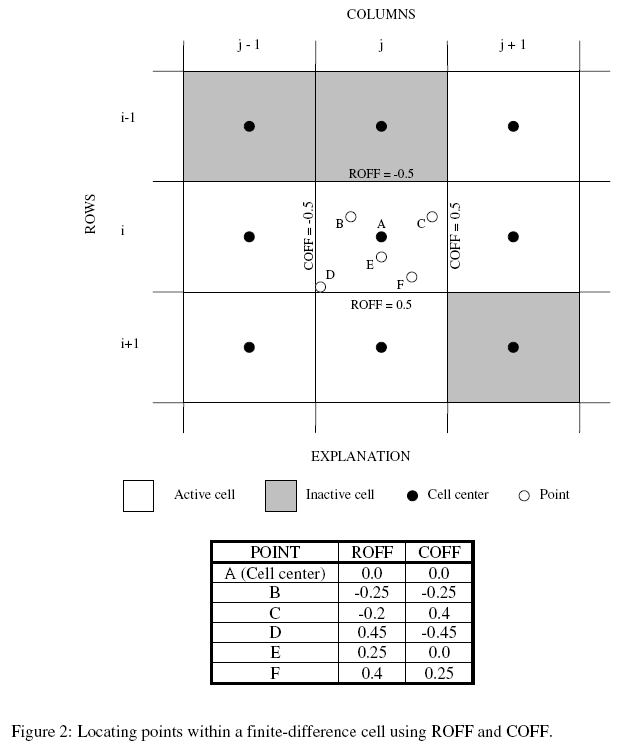
SROFF – is the row offset used to locate the initial location within the finite-difference cell (must range between –0.5 and 0.5; see fig. 2 of Hill and others, 2000).
|
SCOFF – is the column offset used to locate the initial location within the finite-difference cell (must range between –0.5 and 0.5; see fig. 2 of Hill and others, 2000).
|
|
|
Data Set 4
|
OBSNAM LAY ROW COL LOFF ROFF COFF XSTAT IXSTAT YSTAT IYSTAT ZSTAT IZSTAT TADV PLOT-SYMBOL
Item 4 is repeated for each advective-transport observation point to be defined along the path (that is, NPNT times).
OBSNAM – is a string of 1 to 12 nonblank characters used to identify the observation. The identifier need not be unique; however, identification of observations in the output files is facilitated if each observation is given a unique OBSNAM. The current version of MODFLOW-2000 (v 1.17.02) accepts duplicate observation names, but if duplicate names are found, a warning concerning the duplication is written to the Global file.
|
LAY – is the layer of the advective-transport observation.
|
ROW – is the row of the advective-transport observation.
|
COL – is the column of the advective-transport observation.
|
LOFF – is the layer offset used to locate the advective-transport observation within the finite-difference cell (must range between –0.5 at the bottom of the layer and 0.5 at the top of the layer).
|
ROFF – is the row offset used to locate the advective-transport observation within the finite-difference cell (must range between –0.5 and 0.5; see fig. 2 of Hill and others, 2000).
|
COFF – is the column offset used to locate the advective-transport observation within the finite-difference cell (must range between –0.5 and 0.5; see fig. 2 of Hill and others, 2000).
|
XSTAT, YSTAT, ZSTAT – are values from which the weights of the observed locations are calculated depending on how IXSTAT, IYSTAT, and IZSTAT are set.
|
IXSTAT, IYSTAT, IZSTAT – are flags to indicate what XSTAT, YSTAT, and ZSTAT are and how the observation weights are calculated. If the variable STATISTIC represents XSTAT, YSTAT, or ZSTAT and the variable STAT-FLAG represents IXSTAT, IYSTAT, or IZSTAT, respectively, the following definitions apply:
| • | STAT-FLAG = 0, STATISTIC is a scaled variance [L2], weight = 1/STATISTIC, |
| • | STAT-FLAG = 1, STATISTIC is a scaled standard deviation [L], weight = 1/STATISTIC2, and |
| • | STAT-FLAG = 2, STATISTIC is a scaled coefficient of variation [dimensionless], weight = 1/(STATISTIC × Observation value)2. The observation value is calculated as the distance in the x-, y-, or z-coordinate directions between particle starting position, as defined in input item 3, and the observation positions, as defined in item 4. |
|
XSTAT, YSTAT, ZSTAT – are values from which the weights of the observed locations are calculated depending on how IXSTAT, IYSTAT, and IZSTAT are set.
|
XSTAT, YSTAT, ZSTAT – are values from which the weights of the observed locations are calculated depending on how IXSTAT, IYSTAT, and IZSTAT are set.
|
TADV – is the time of this advective-front observation, relative to the beginning of the steady-state simulation, in consistent units.
|
PLOT-SYMBOL – is an integer that is written to output files intended for graphical analysis to allow control of the symbols used to plot data.
|
|
|
Data Set 5
|
IOWTQAD – is a flag indicating whether a full weight matrix will be specified.
| • | If IOWTQAD ≤0, a full weight matrix will not be specified and the STATISTIC values in ITEM 4 will be used to calculate weights. |
| • | If IOWTQAD > 0, a full weight matrix will be specified. |
|
|
Items 6-7 are required if IOWTQAD>0.
|
Data Set 6
|
FMTIN IPRN
FMTIN—is the Fortran format to be used in reading each line of the variance-covariance matrix used to calculate the weighting. The format needs to be enclosed in parentheses and needs to accommodate real numbers.
|
IPRN—is a flag identifying the format in which the variance-covariance matrix is printed. If IPRN is less than zero, the matrix is not printed. Permissible values of IPRN and corresponding formats are:
|
|
|
|
|
|
|
|
1
|
10G12.3
|
6
|
5G12.3
|
2
|
10G12.4
|
7
|
5G12.4
|
3
|
9G12.5
|
8
|
5G12.5
|
4
|
8G13.6
|
9
|
4G13.6
|
5
|
8G14.7
|
10
|
4G14.7
|
|
|
|
Data Set 7
|
WTQ(NTT2,NTT2) (format FMTIN)
WTQ—is an array containing the variance-covariance matrix on advective-transport observations [L 2 ]. The array is square with dimensions equal to the total number of advective-transport observations (for example, NLOC times two if the tracking is two dimensional or three if the tracking is three dimensional) and for each observation location is entered in the order X, Y, and Z, if applicable. For elements WTQ(I,J), if I ≠J, WTQ(I,J) is the covariance between observations I and J; if I = J, WTQ(I,J) is the variance of observation I. Note that the variance-covariance matrix is symmetric, but the entire matrix (upper and lower parts) must be entered.
|
|