
Drainage Area
What Does “Drainage Area” Mean?
Rain falls on a landscape and flows downhill. The land that delivers surface water to a common outlet — a gage, a confluence, or a lake where water leaves the basin — is the drainage area of that outlet. The boundary separating one drainage area from its neighbors is a drainage divide, the line along which surface water could flow in either direction. These concepts are old and well-established; the USGS has been delineating and coding hydrologic boundaries in digital form since the mid-1980s, and the underlying ideas go back much further. An introduction is available from the USGS Water Science School .
Drainage area underpins much of applied hydrology. Unit-area runoff, flood frequency estimates, flow statistics, and water-balance calculations all depend on it. When an analysis reports streamflow in volume per area, the denominator is a drainage area — and the specific value of that drainage area depends on the dataset and method used to determine it. The USGS definition of drainage area specifies that reported values are “measured using the most accurate maps available” and that accuracy varies with input data 2006 Water Data Report Definitions .
This discussion focuses on drainage areas of natural systems and differences that arise from derivation using different digital data sources. Human-modified drainage systems likely pose greater challenges in delineation and are not discussed here. The sections that follow describe routine and unexpected examples from five drainage basins to show the diversity of outcomes and how that diversity is connected to the hydrologic landscape and the digital data sources used.
Multiple federal datasets report drainage area for the same locations, and for most of those locations the values closely agree. Where the reported values diverge among datasets, the physical landscape drives the divergence.
Where Drainage Area Is Well-Determined
The French Broad River at Asheville, North Carolina (USGS streamgage 03451500 ) drains roughly 2,447 sq km of Appalachian terrain. Steep ridges, connected perennial channels, and no internally drained areas make this basin’s drainage area well-determined. The process to determine drainage area is mechanical: locate the outlet’s hydrologic location (pour point), trace the topographic divide along ridgelines, and compute the enclosed area. Where topographic relief is strong — where elevation gradients and changes in slope are sharply defined — the result depends very little on which dataset or method produces it.
The examples on this page draw drainage area values from four sources. The National Hydrography Dataset Plus version 2 (NHDPlusV2) provides network-accumulated catchment areas along connected flowlines. The Watershed Boundary Dataset (WBD) provides hydrologic unit boundaries at multiple scales — HU12, HU10, and HU8 — along with type designations and area attributes. NHDPlus High Resolution (NHDPlusHR) provides a finer-scale network and catchment delineation. The National Water Information System (NWIS) carries gage-level drainage area values reported by USGS field offices.
Table 1. Drainage area estimates for the French Broad River at Asheville.
| Source | Area (sq km) |
|---|---|
| Network DA (NHDPlusV2) | 2,446.9 |
| HU12 DA | 2,446.0 |
| HU10 DA | 2,446.0 |
| NWIS drainage_area | 2,447.5 |
The numbers confirm this. Four independent sources — accumulated NHDPlusV2 catchment areas, HU12 and HU10 boundaries from the WBD, and the NWIS gage record — all fall within 1.5 sq km of one another across a basin of nearly 2,500 sq km.
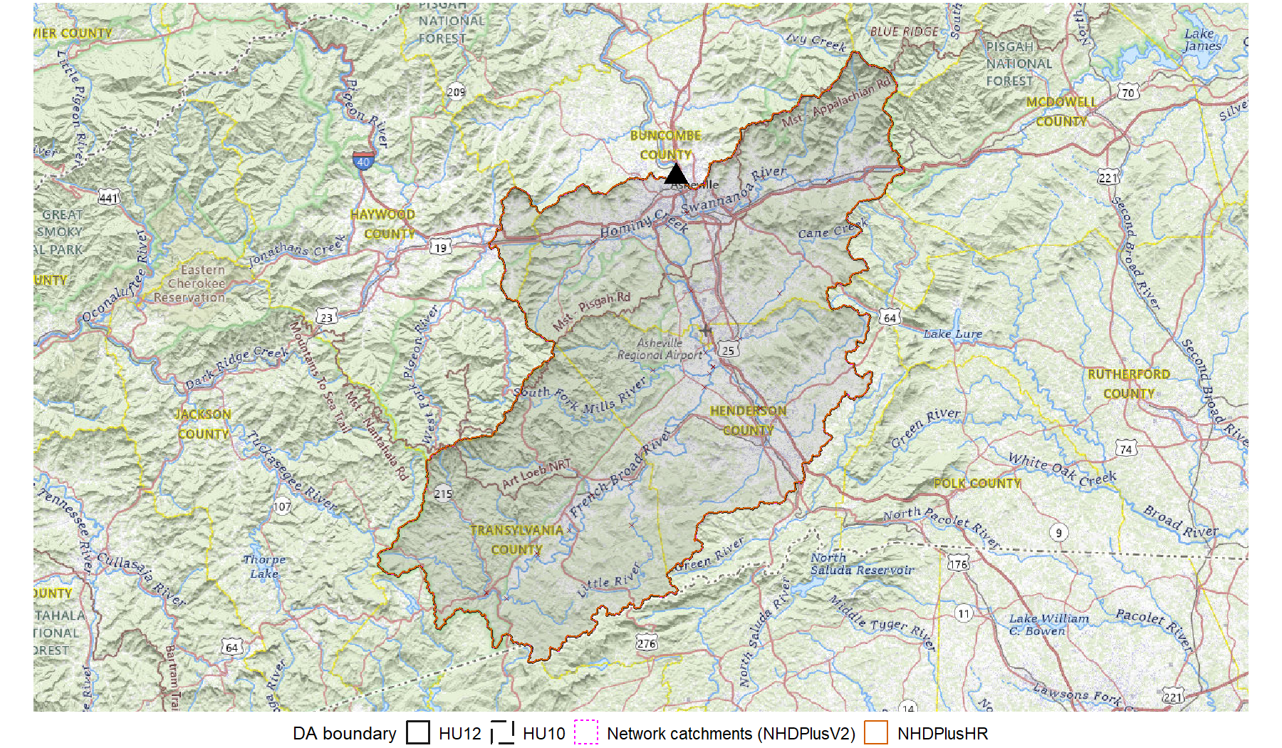
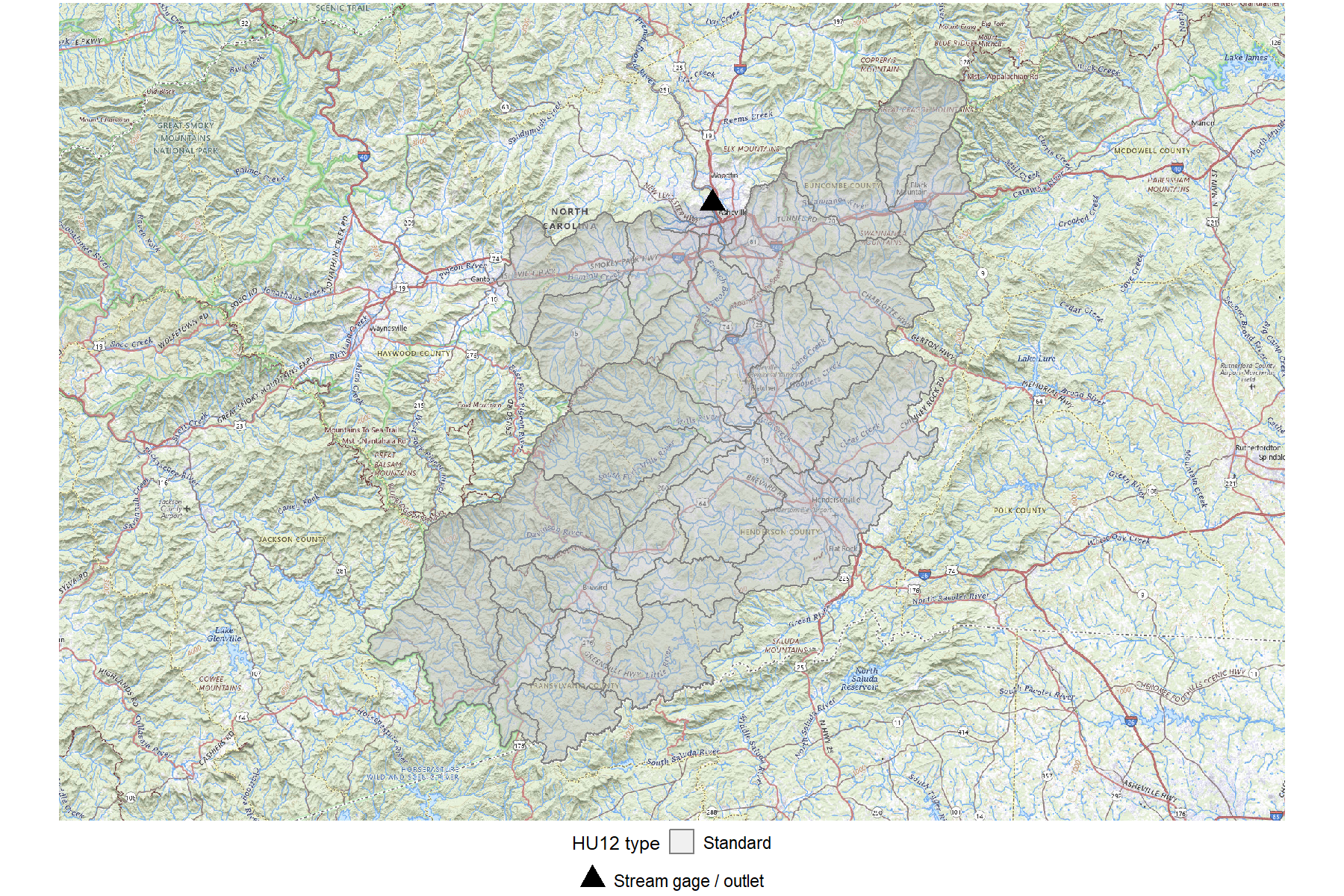
The boundary map shows why. In the southern Appalachians, ridgelines are pronounced and divides are unambiguous — the HU10, HU12, and network-derived boundaries trace nearly the same line. The HU12 type map below reinforces this from a different angle. The WBD assigns each HU12 a type designation: Standard (drains to a downstream HU12 through normal surface flow), Closed basin (no surface outlet), Multiple outlets (more than one outlet within the same downstream system), Frontal (drains directly to a coast or large water body), or Water (an open-water body). Every HU12 in the French Broad basin is Standard.
Convergence like this is the norm for basins in well-drained terrain with strong topographic relief. The conditions that produce varied drainage area estimates — flat terrain, internal drainage, ephemeral flow — are the subject of the sections that follow.
Two Numbers, Not One: Total and Contributing Drainage Area
Not all land inside a topographic boundary delivers surface runoff to the outlet. Closed depressions — playas, salt flats, prairie potholes — retain water internally. Under typical conditions, runoff that enters these low-lying areas does not reach a downstream channel network; it leaves only by evaporation or subsurface seepage. The land they occupy sits inside the drainage basin but does not contribute to streamflow at the outlet. Federal datasets call this noncontributing area.
Federal datasets have long recognized the distinction. The Watershed Boundary Dataset includes two area attributes at each hydrologic unit level: AreaSqKm (total drainage area) and NonContributingAreaSqKm which are also represented at HU12 and coarser units (HU10, HU8) through hydrologic unit type designations and the upstream downstream relationships among units (Jones and others, 2022, TM 11-A3
). A “closed” HU12 is within a larger unit so while it is not surface connected to a downstream neighbor, it can still be lumped into a broader basin. NWIS site records carry a similar pair: drainage_area (total) and contributing_drainage_area. The USGS Water Resources Mission Area definition
specifies that total drainage area includes all closed basins within the boundary unless otherwise noted. Contributing drainage area is the complement — total area minus the noncontributing portion.
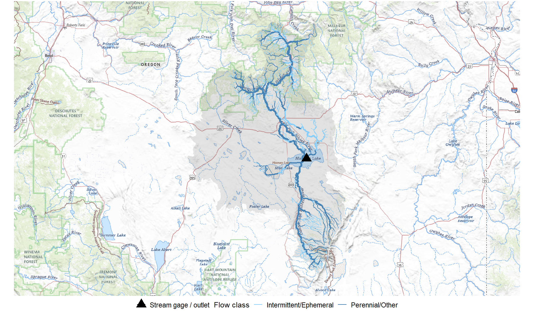
A drainage basin with no surface outlet at all is an endorheic basin (also called a closed basin). Water enters but does not leave as surface flow. The Harney Basin in southeastern Oregon — home to Malheur and Harney Lakes — is one such system. The Silvies River and the Donner und Blitzen River flow into these lakes, but no channel carries water out. The basin is the complete case of noncontributing area: from the perspective of any downstream system, the entire basin is noncontributing.
The drainage area numbers for the basin contributing to Malheur Lake reflect this condition:
Table 2. Drainage area estimates for the Malheur Lake drainage basin.
| Source | Area (sq km) |
|---|---|
| Network DA (NHDPlusV2) | 4,585.6 |
| HU12 DA | 7,307.9 |
| HU10 DA | 8,543.9 |
| HU8 DA | 12,287.4 |
The network-derived drainage area — accumulated from NHDPlusV2 catchments along connected flowlines — covers 4,586 sq km. The HU12 boundaries encompass 7,308 sq km, more than 50 percent larger than the network value. The HU8 envelope reaches 12,287 sq km, nearly three times the network area. These are not disagreeing answers to the same question; they answer different questions. The network accumulation follows connected flowlines and stops where surface connectivity ends. The HU boundaries delineate the full topographic extent of the basin, including land that drains internally.
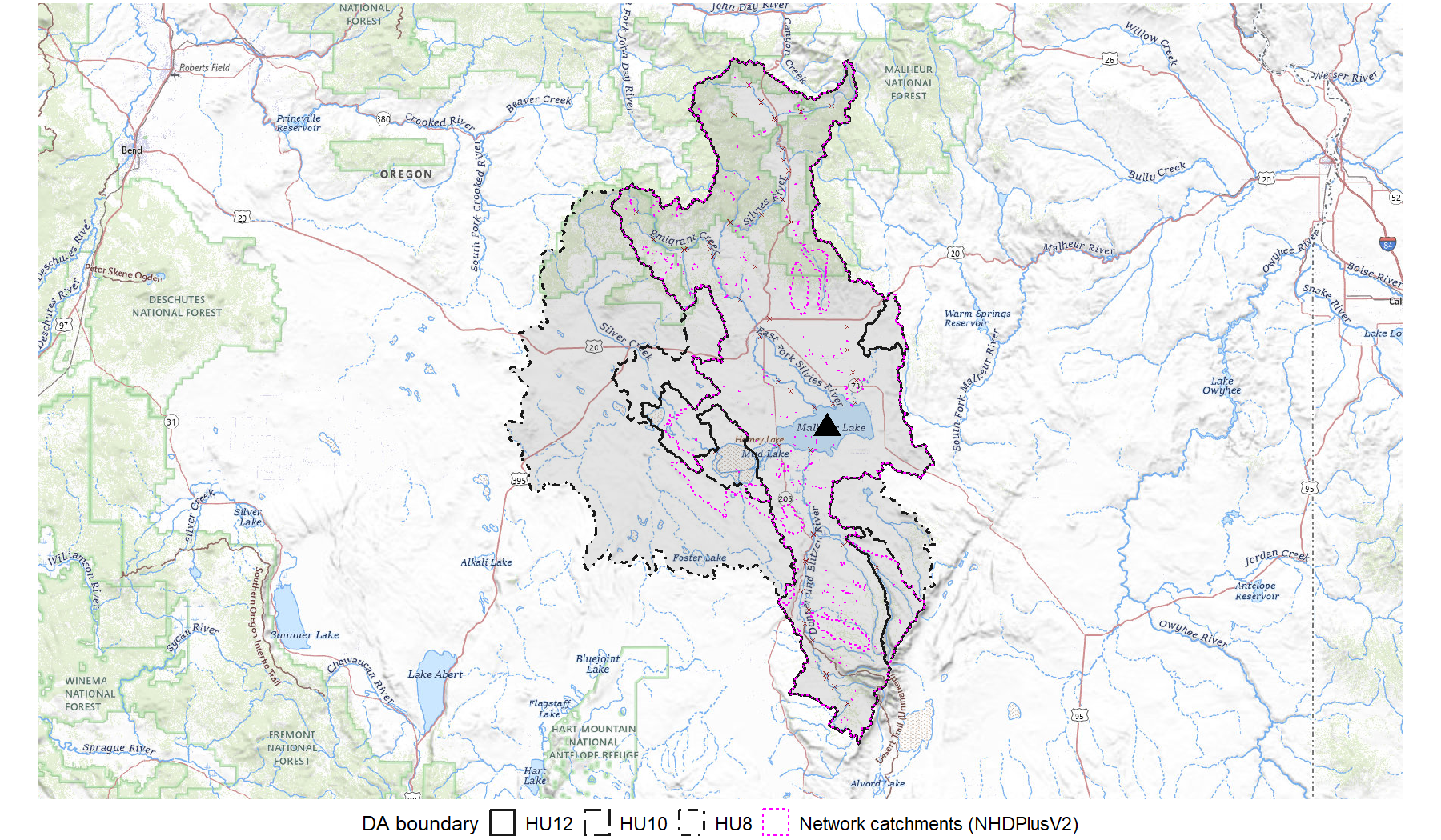
The HU12 type map shows the two reported numbers — total drainage area and contributing drainage area — as categorical designations rather than as a single numeric ratio. Mud Lake appears as a Water HU12 (blue). Malheur Lake and the pluvial-lake margins are Closed-basin HU12s (brown), where surface drainage terminates without reaching a downstream unit. Multiple-outlet HU12s (grey) sit on the low-gradient flats of the Harney Basin where drainage can split between more than one downstream unit. The surrounding Standard HU12s (light grey) supply the Silvies River and Donner und Blitzen River corridors that actually reach the lake.
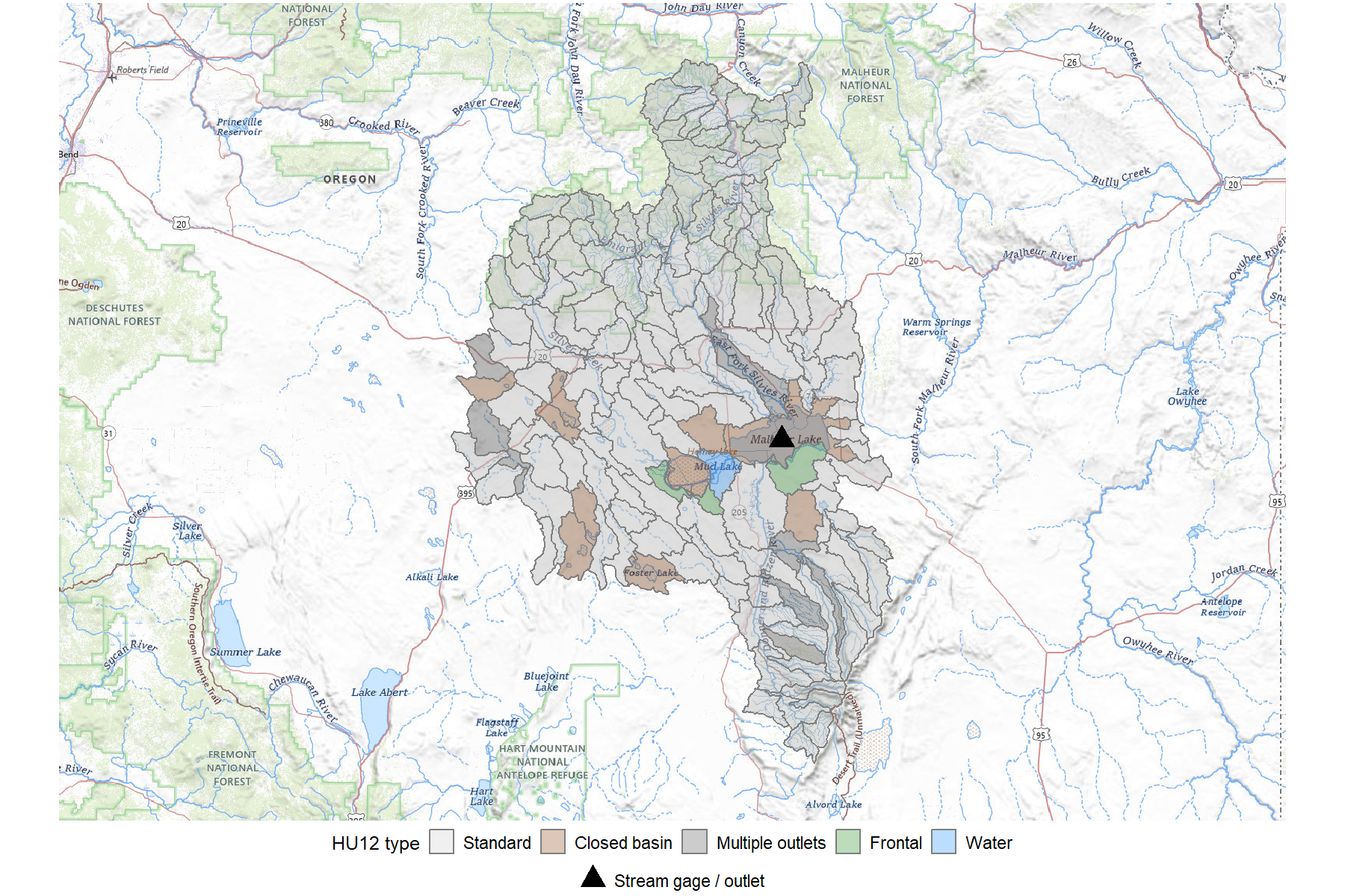
Two perennial corridors deliver surface flow to Malheur Lake — the Silvies River from the north and the Donner und Blitzen from the south. The western lobe of the HU8 envelope contains no perennial connection to the lake; it belongs to the adjacent Silver Creek-Silver Lake closed basin, included because NHDPlusV2 retains a network link between the two endorheic systems. The HU8 number reflects this limit of network-walked aggregation at coarse units: adjacent closed basins can lump together when even a sparse channel connection exists between them.
The Harney Basin is an extreme case — a fully endorheic system — but the two-number pattern it illustrates applies broadly. Any basin with closed depressions, internally drained flats, or areas of uncertain surface connectivity may show some gap between total and contributing drainage area. The mechanisms that create that gap are the subject of the next section.
Where Estimates Diverge — and Why
When topographic relief dominates, drainage area methods converge — the French Broad showed this. When the relief weakens — flat terrain, noncontributing area in glaciated landscapes, ephemeral flow — the range of defensible drainage area values widens. The Harney Basin represents the end member, where all three conditions operate together. The examples that follow isolate three distinct mechanisms, each producing divergence for a different physical reason.
Flat Terrain and Boundary Placement
A drainage divide in steep terrain falls along a ridge where elevation gradients point unambiguously in opposite directions. In flat terrain — a few meters of elevation change over tens of kilometers — the gradient weakens. Changes in elevation data, processing method, or boundary delineation rules can shift the divide by kilometers — and with it, the drainage area of every downstream location.
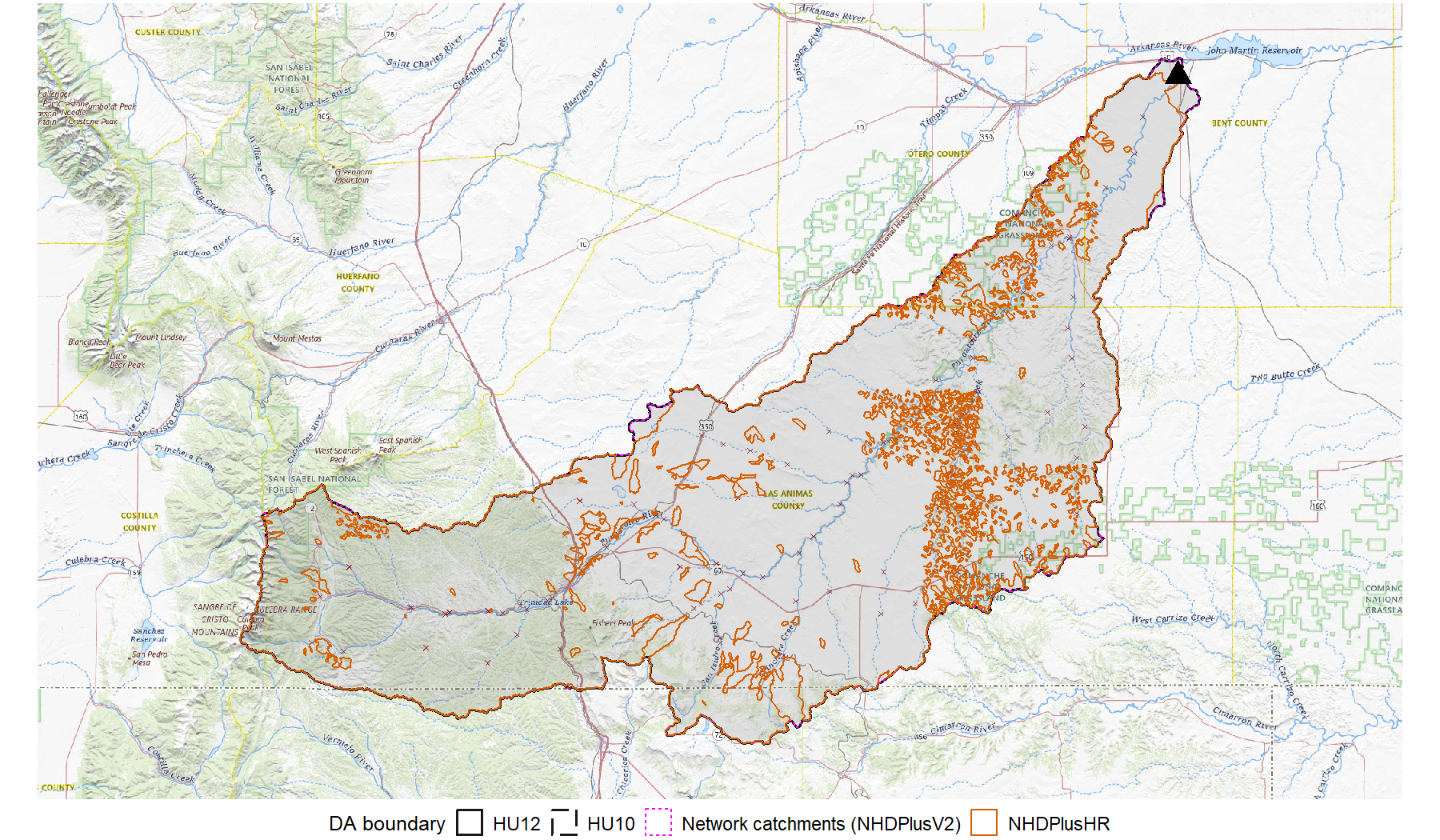
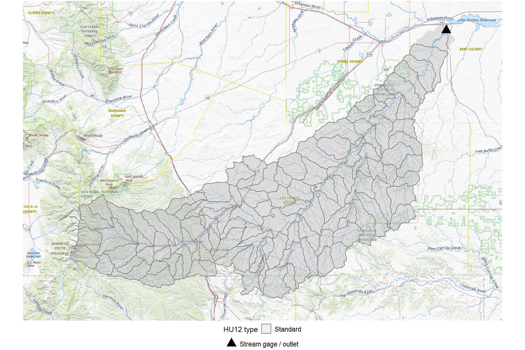
A well-documented case appears in the Purgatoire River basin in southeastern Colorado. Dupree and Crowfoot (2012, TM 11-C6) compared drainage areas derived by manual delineation from USGS topographic maps with GIS-derived areas for 518 basins across Colorado. For the Purgatoire River near Las Animas (USGS streamgage 07128500 ), the manual method yielded 3,318 sq mi (8,594 sq km) and the GIS method yielded 3,441 sq mi (8,912 sq km) — a difference of 123 sq mi (319 sq km). A noncontributing area adjacent to the basin had been included in the traditional delineation but was placed in the neighboring hydrologic unit to the west by the Watershed Boundary Dataset. The same 123 sq mi difference propagated to five additional downstream gages on the Purgatoire and Van Bremer Arroyo.
The example data for this gage show the downstream consequences of that boundary placement:
Table 3. Drainage area estimates for the Purgatoire River near Las Animas.
| Source | Area (sq km) |
|---|---|
| TM 11-C6 manual | 8,594 |
| TM 11-C6 GIS | 8,912 |
| Network DA (NHDPlusV2) | 8,930.0 |
| HU12 DA | 8,875.0 |
| HU10 DA | 8,875.0 |
| NHDPlus HR DA | 8,217.8 |
| NWIS drainage_area | 8,912.2 |
| NWIS contributing_drainage_area | 8,881.6 |
The NHDPlusV2 network, HU12, HU10, and NWIS values all converge near 8,900 sq km — within 18 sq km of the TM 11-C6 GIS value. The network accumulation and the HU boundaries agree because one was built to match the other: NHDPlusV2 wall-burned (imposed as artificial elevation barriers) WBD boundary lines into its elevation data, inheriting the WBD’s placement of the disputed area.
The Purgatoire headwaters drain the Sangre de Cristo Mountains and the Spanish Peaks — steep terrain where all boundary sources agree. Downstream, the river crosses into the high plains of southeastern Colorado. Dupree and Crowfoot reported that the disputed noncontributing area sat adjacent to the basin’s western margin — “not a part of the Purgatoire hydrologic unit nor a part of the hydrologic unit to the west.” The manual method included it in the Purgatoire drainage; the WBD assigned it to the neighboring unit. The 319 sq km difference — about 3.6 percent of the basin’s total area — between those two placements is what Dupree and Crowfoot documented — the divide sits in terrain flat enough that two defensible methods put it in different places.
The NHDPlus HR value introduces a separate divergence. At 8,218 sq km — 712 sq km below NHDPlusV2 — the HR shortfall does not trace to boundary placement. The boundary figure shows HR catchment gaps scattered through the flat central and southeastern interior, where the high-resolution network is sparse and disconnected. Where HR processing finds no connected flowline path, those catchments drop out of the accumulated drainage area — the same network-disconnection mechanism visible in the James River example in the next section.
Boundary placement uncertainty — the condition Dupree and Crowfoot described — arises wherever gradients are small enough that the divide could reasonably fall in more than one place. The Purgatoire basin adds a second layer: flat terrain also produces sparse, disconnected networks in the high-resolution data, and those disconnections reduce the accumulated drainage area independently of where the divide falls.
Noncontributing Area in Glaciated Landscapes
Boundary placement uncertainty affects where the divide falls. A different mechanism affects how much of the land inside that divide actually contributes flow: closed depressions that store runoff locally, releasing it downstream only when they fill and spill over. Under dry conditions, water that enters a depression stays there. Under wet conditions — sustained rainfall, snowmelt, high background moisture — depressions overtop into the next one downslope and eventually connect to the channel network. The contributing fraction of drainage area in these landscapes is not fixed; it varies with hydrologic conditions. In the prairie pothole region of the northern Great Plains, glacial drift created thousands of such depressions — potholes — scattered across an otherwise low-gradient landscape.
The James River near Grace City, North Dakota (USGS streamgage 06468000 ) illustrates this pattern. The basin sits in the heart of the prairie pothole region, and the drainage area values from different sources diverge accordingly:
Table 4. Drainage area estimates for the James River near Grace City.
| Source | Area (sq km) |
|---|---|
| Network DA (NHDPlusV2) | 1,442.4 |
| HU12 DA | 1,436.6 |
| HU10 DA | 1,655.5 |
| NHDPlus HR DA | 620.4 |
| NWIS drainage_area | 1,849.3 |
| NWIS contributing_drainage_area | 722.6 |
The HU10 boundary encompasses 1,656 sq km — roughly 220 sq km more than the HU12 boundary. HU12s nest within HU10s, so the difference is not in boundary geometry but in which HU12s are included: the HU10 unit includes additional pothole sub-basins along the margins that do not aggregate into the gage’s HU12 drainage. The NHDPlus HR drainage area, at 620 sq km, is less than half the network value. This reflects how the high-resolution network handles the disconnected pothole terrain: where the HR processing finds no connected path, those catchments drop out of the accumulated area.
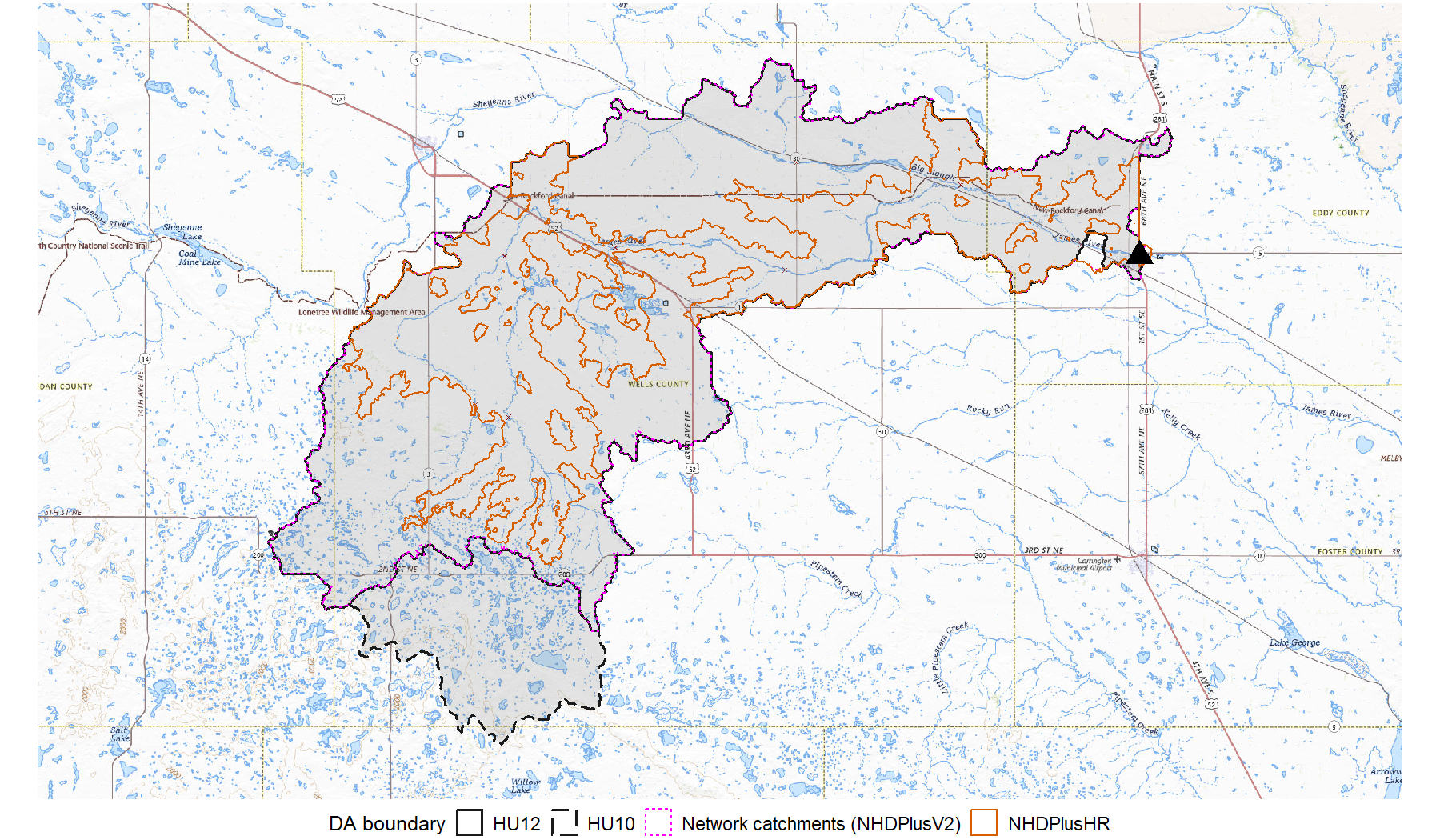
The network map shows the mechanism. The lower main stem of the James River is perennial — a connected channel carrying flow year-round. The upper basin and its tributaries are intermittent, threading through a landscape dotted with small lakes and closed depressions. Whether a given pothole contributes to downstream flow in a given year depends on how much water it received and how much it already held.
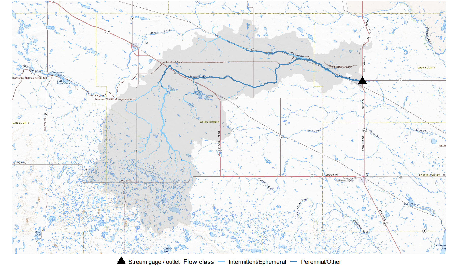
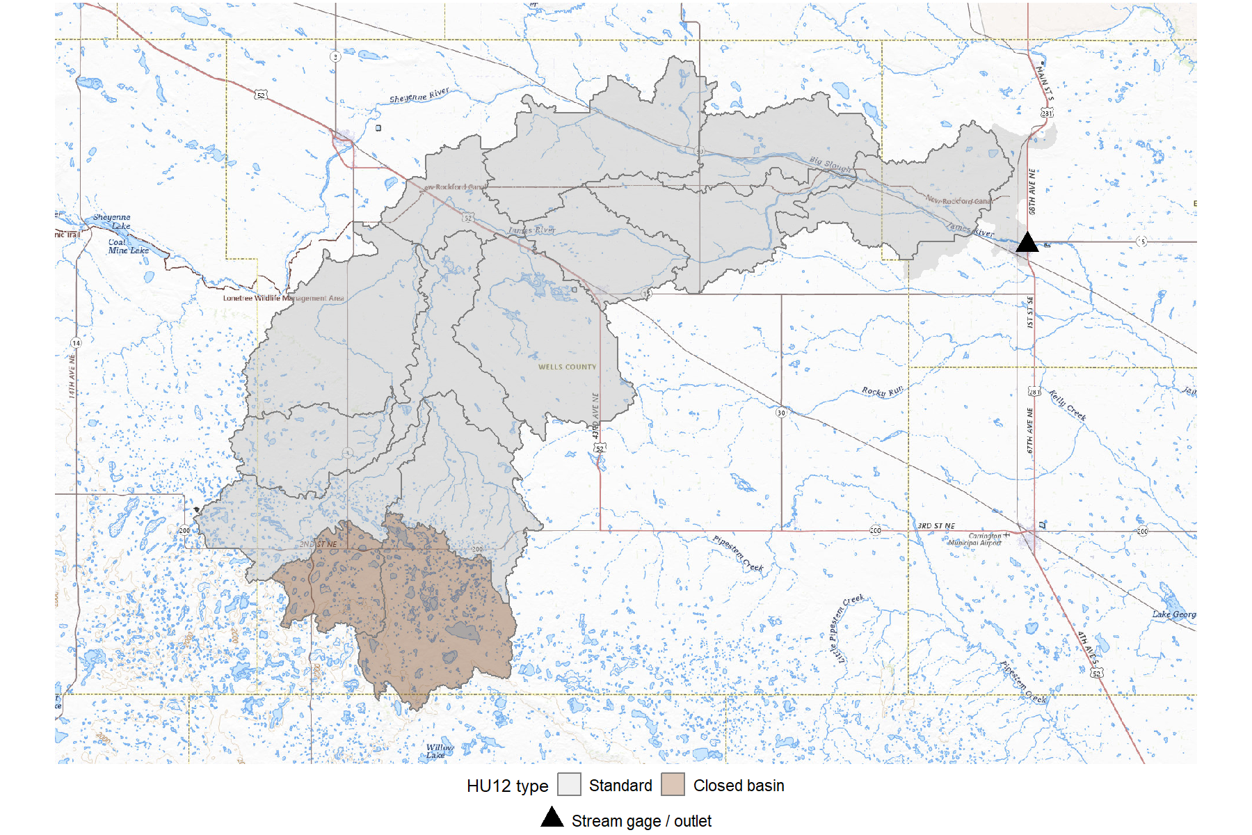
The HU12 type attribute captures only a small part of the pothole story. The WBD flags just two closed-basin units in the upper headwaters; every other HU12 in the basin is Standard. The broader pothole-storage pattern shows up instead in the boundary comparisons — the HU10 boundary reaches further south than the HU12 and network boundaries — and especially in the NHDPlus HR value, where network disconnections in pothole terrain produce a dramatically smaller accumulated area. The signature in the numbers is a large gap between NWIS total and contributing drainage area, paired with an NHDPlus HR value far below the network total — both reflecting terrain where surface connectivity is intermittent rather than permanent. How contributing area varies with moisture level is a separate question beyond the scope of this page.
Ephemeral Flow and Transmission Losses
Prairie potholes store water in closed depressions. A different mechanism operates in arid landscapes: water enters a channel but does not reach the downstream network. Channels in these regions flow only during and shortly after rainfall — ephemeral flow — and water that does enter the channel may be lost to infiltration through the streambed before it arrives at the next downstream reach. These are transmission losses, and they reduce the effective contributing area below what the topographic boundary would suggest.
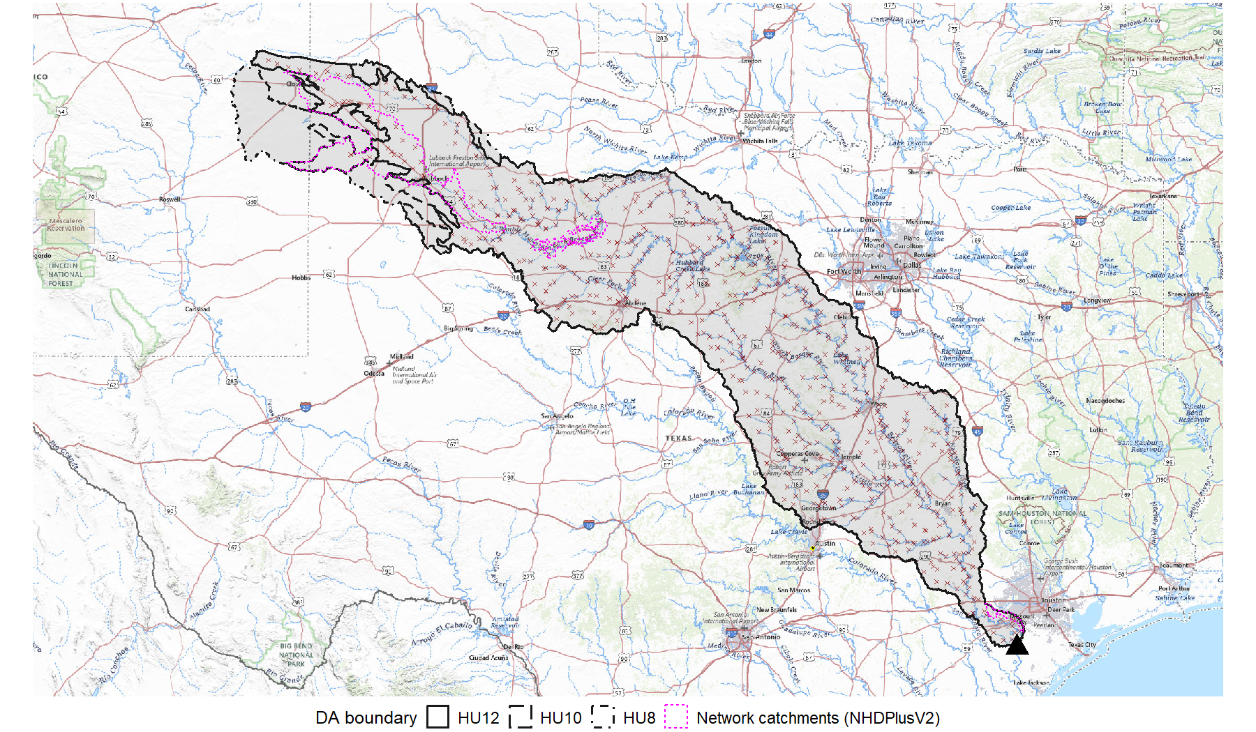
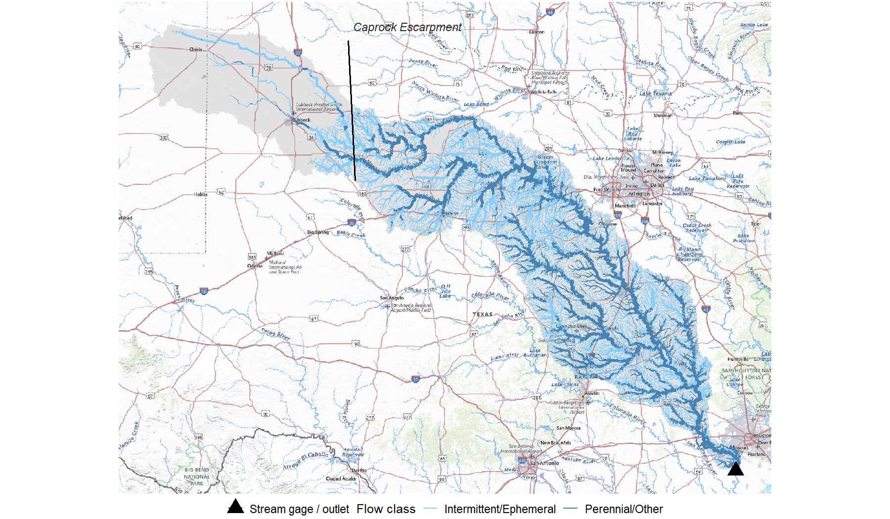
The Brazos River at Rosharon, Texas (USGS streamgage 08116650 ) spans the transition from arid western uplands to relatively moist eastern plains. The Caprock Escarpment — a prominent physiographic boundary running roughly north-south through the Texas Panhandle — marks the divide between these two regimes (Wermund, 1996 ). West of the escarpment, channels are ephemeral, precipitation is sparse, and transmission losses are high. East of it, the network becomes perennial and well-connected — a contrast documented by gain/loss measurements along the Brazos main stem in Baldys and Schalla (2016, SIR 2011-5224) .
Table 5. Drainage area estimates for the Brazos River at Rosharon.
| Source | Area (sq km) |
|---|---|
| Network DA (NHDPlusV2) | 103,578.2 |
| HU12 DA | 99,673.5 |
| HU10 DA | 108,940.1 |
| HU8 DA | 118,108.1 |
| NWIS drainage_area | 117,427.6 |
| NWIS contributing_drainage_area | 92,651.7 |
The divergence appears most strongly at coarser scales: the HU8 envelope, at 118,108 sq km, exceeds the network drainage area by more than 14,500 sq km. That difference reflects the western uplands where HU boundaries follow topographic divides into arid terrain that the network accumulation does not fully reach. The gage’s NWIS record carries the same disagreement in a different form — drainage_area reports 117,428 sq km while contributing_drainage_area reports 92,652 sq km, a gap of nearly 25,000 sq km that the HU12 total does not resolve.
The network map shows the two regimes. West of the Caprock Escarpment, the network is sparse — intermittent and ephemeral reaches thread through the high plains with wide gaps between channels. East of it, the network thickens into a dense perennial system draining toward the Gulf Coast. The shift from sparse ephemeral coverage to dense perennial network tracks the escarpment closely.
The HU12 type map shows the WBD’s categorical designations across the basin. Closed-basin HU12s (brown) cluster in the arid northwestern uplands of the Llano Estacado, where surface water never reaches the Brazos. Multiple-outlet HU12s (grey) mark units with more than one outlet within the same downstream system — where flow leaves through multiple points rather than a single pour point. Frontal HU12s (green) appear near the coast where catchments drain directly to the coast rather than to a downstream HU12.1 Standard HU12s (light grey) dominate the perennial eastern main stem. The ephemeral-disconnection pattern along the western tributaries is not captured at HU12 type. It shows up instead in the boundary divergence, in the HU8 envelope, and in the NWIS contributing-area value.
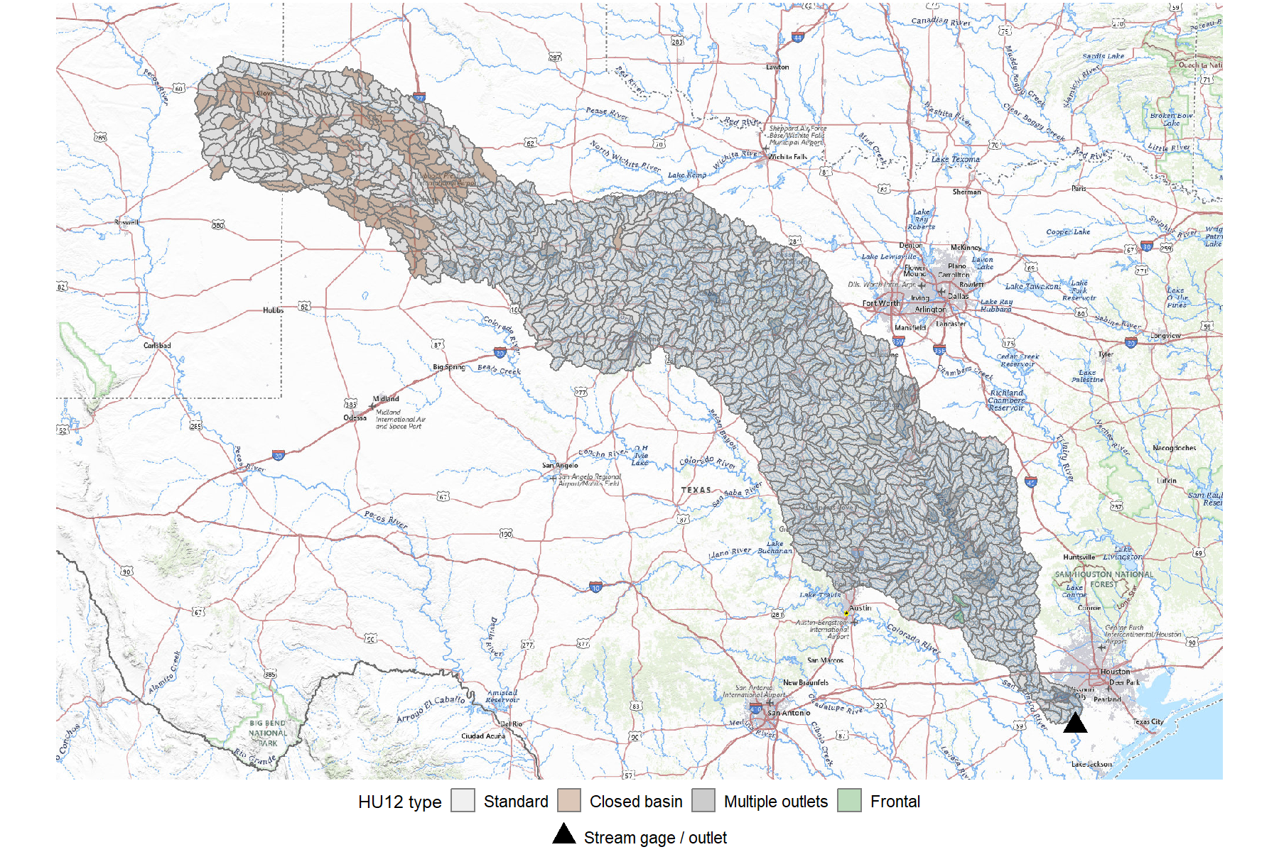
The indicator of non-permanent flow in the numbers is the large gap between the HU8 envelope and the NWIS contributing drainage area — reflecting land that sits inside the topographic boundary but does not always deliver surface water to the outlet.
1 The WBD also assigns Frontal designations to several HU12s in the central basin — not only near the coast. These interior Frontal units drain directly to large reservoirs or mainstem water bodies rather than to a downstream HU12 through a channel network.
How Datasets Encode These Realities
The physical mechanisms described above — boundary placement uncertainty, internal storage, transmission losses — exist in the landscape regardless of how datasets represent them. The datasets that practitioners use to compute drainage area encode these realities through a chain of processing choices, each reasonable, each carrying consequences for the resulting numbers and the determinations they represent.
As shown in the HU12 Types maps above, the Watershed Boundary Dataset documents closed-basin and related designations through hydrologic unit type attributes and through the way smaller units nest inside larger ones. These designations reflect determinations made during boundary delineation — which land drains where, which depressions are treated as closed, which areas are assigned to which hydrologic unit. A standard-type HU12 inside a closed HU8 is part of that larger unit’s drainage area without being surface-connected to anywhere beyond it; the type and hierarchy together carry the information that a single area attribute would not.
NHDPlusV2 used WBD HU12 boundary lines as “walls” during hydro-enforcement of the National Elevation Dataset — artificially raising elevation values along those boundaries so that catchment delineations would coincide with hydrologic unit boundaries (NHDPlusV2 User Guide, v2.1 ). NHDPlus HR applies a similar technique, creating virtual walls at WBD divides and virtual trenches at stream locations to produce catchments that agree with both the hydrography and the WBD boundaries (Moore and others, 2025, SIR 2025-5031 ). As a result, NHDPlus-derived drainage areas reflect both the terrain surface and the WBD’s boundary determinations — including its treatment of noncontributing areas and divides subject to boundary placement uncertainty.
Network disconnections add a further source of variation. In NHDPlusV2, gaps in the connected network can produce catchment “holes” — areas that fall within the topographic boundary but are not reached by network tracing. Whether an analysis retains or fills these holes affects the resulting drainage area, and different tools may handle it differently without making the choice visible to the user.
Living With Diverse Estimates
The examples on this page show drainage area values that range from near-perfect agreement — less than 1 sq km across three sources for the French Broad — to differences of thousands of square kilometers for the Brazos and the Harney Basin. In each case the divergence traces to a physical mechanism interacting with the methods a given dataset uses to represent it. Flat terrain produces boundary placement uncertainty in the Purgatoire basin. Glacial potholes produce variable contributing fractions along the James River. Ephemeral channels and transmission losses produce a gap between topographic and effective contributing area across the western Brazos.
These mechanisms arise from the terrain and channel characteristics of each landscape, and the datasets that encode them do so through documented processing steps — boundary delineation rules, hydro-enforcement techniques, network connectivity determinations. Adopting a dataset for analysis means working with the drainage area values that those processing steps produced. Understanding what drove a particular value — and how it might differ under a different dataset or method — is part of working with drainage area at scale.
The distinction between total and contributing drainage area exists because different applications need different quantities. A flood frequency analysis may need total drainage area; a water-balance model may need contributing drainage area. NWIS records both at the gage level; the WBD carries the same distinction through hydrologic unit types and the aggregation hierarchy. Documenting which dataset, version, and method were used to produce a value preserves information that collapsing to a single number would discard.