 (C1)
(C1)
The governing equation for the main channel is given by:
(C1)
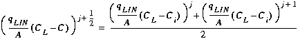
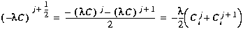
where L[C] is the finite difference approximation of the advection and dispersion terms, as given in Appendix B. In order to attain second order accuracy in both time and space, Equation (C1) is evaluated at the intermediate time level, j+1/2. To this end, the time derivative is approximated at the intermediate time level using a centered finite difference:
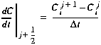 (C2)
(C2)
where
Furthermore, the right-hand side at j+1/2 is simply the average of the terms evaluated at times j and j+1. Combining this average with Equation (C2), Equation (C1) becomes:
t
the integration time step [T] j denotes the value of a parameter or variable at the current time j+1 denotes the value of a parameter or variable at the advanced time
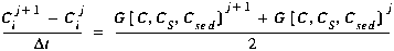 (C3)
(C3)
where
 (C4)
(C4)
Because Equation (C3) is dependent on the solute concentrations in the neighboring segments at the advanced time level (Ci-1, Ci+1 at time j+1), it is not possible to explicitly solve for Cij+1. In the sections that follow, Equation (C3) is rearranged so that all of the known quantities (i.e. those at time j) appear on the right-hand side and all of the unknown quantities (i.e. those at time j+1) appear on the left. This rearrangement yields:
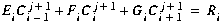 (C5)
(C5)
where E, F and G are matrix coefficients and R is a forcing function.
We now proceed to develop the matrix coefficients and the forcing function by examining each term in Equation (C3). In general, unknown quantities in each term contribute to the matrix coefficients while known quantities make up the forcing function. After going through each term, individual contributions are summed (see Section C4.0) to obtain E, F, G and R.
 (C6)
(C6)
 (C7)
(C7)
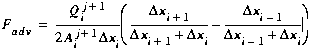
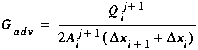
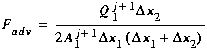
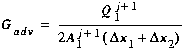
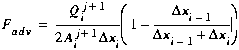
Using the finite difference equations for the advection term (Equations (B7), (B11), and (B17)), we develop the contributions to the matrix coefficients shown below. Note that due to the presence of boundary conditions, the contributions depend on the type of segment for which Equation (C5) is developed.
 (C8)
(C8)
 (C9)
(C9)
 (C10)
(C10)
 (C11)
(C11)
 (C12)
(C12)
 (C13)
(C13)
 (C14)
(C14)
 (C15)
(C15)
 (C16)
(C16)
 (C17)
(C17)
 (C18)
(C18)
 (C19)
(C19)
 (C20)
(C20)
 (C21)
(C21)
 (C22)
(C22)
 (C23)
(C23)
 (C24)
(C24)
 (C25)
(C25)
 (C26)
(C26)
 (C27)
(C27)
 (C28)
(C28)
The contributions are thus:
 (C29)
(C29)
 (C30)
(C30)
 (C31)
(C31)
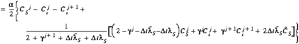
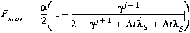
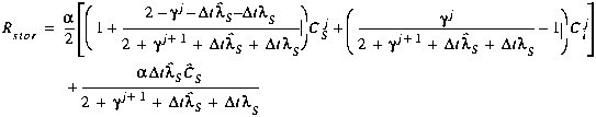
To decouple the governing transport equations (see Section 3.4.5), Equation (19) is used to eliminate CSj+1. Equation (C31) thus becomes:
 (C32)
(C32)
The contributions to the matrix coefficients are given by:
 (C33)
(C33)
 (C34)
(C34)
 (C35)
(C35)
To decouple the governing transport equations (see Section 2.4.5),
the Crank-Nicolson solution of the streambed sediment equation is used
to eliminate  . Equation (C35)
thus becomes:
. Equation (C35)
thus becomes:
 (C36)
(C36)
The contributions to the matrix coefficients are given by:
 (C37)
(C37)
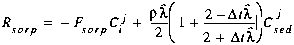 (C38)
(C38)
 (C39)
(C39)
The contributions are given by:
 (C40)
(C40)
 (C41)
(C41)
t:
 (C42)
(C42)
 (C43)
(C43)
 (C44)
(C44)
 (C45)
(C45)