This example uses interpolation for several user-defined data sets. Several different interpolation algorithms are available in ModelMuse. In this section, the effects of changing the interpolation algorithm will be explored. To do this, the grid will be colored using the Kx data set and then the interpolation algorithm for several user-defined data sets will be changed to see how that affects the results. The user may not get identical results to those illustrated for the Nearest interpolation method (fig. 64) and for the Inv.Dist. Sq. interpolation method (fig. 65). This is because the user most likely will not have cells in precisely the same locations as those used to generate figures 64 and 65.
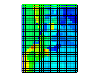
32.Select Data|Data Visualization|Color Grid… Select the Kx data set (Under Data Sets|Required|Hydrology) and click the OK button. After hiding all objects and making the top layer the active layer, the grid should look similar to figure 64.

Figure 64. Distribution of Kx in the top layer of the Biscayne Bay aquifer model when the Nearest interpolation method is used.
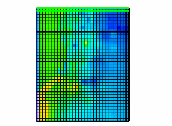
33.Select Data|Edit Data Sets… Select the “Upper_Aquifer_Transmissivity” data set, change its Interpolation to Inv. Dist. Sq. (Inverse distance squared) and click Apply. The grid should look similar to figure 65. The hydraulic conductivity at each element in the upper aquifer is calculated be dividing the interpolated transmissivity by the aquifer thickness. When the interpolation algorithm for the transmissivity is changed, Kx changes too.

Figure 65. Distribution of Kx in the top layer of the Biscayne Bay aquifer model when the Inv. Dist. Sq. interpolation method is used.
34.Next change the interpolation algorithm for “Upper_Aquifer_Transmissivity” to Nearest Point. The appearance of the grid should go back to what it was when the interpolation algorithm was Nearest. This is because the data for “Upper_Aquifer_Transmissivity” consist entirely of point objects. The Nearest Point and Nearest interpolation algorithms give the same results when applied to points, although Nearest Point is faster. They give different results when applied to other sorts of objects. The user can experiment with some of the other interpolation methods to see how the results they give differ from one another.
35.Next try changing the interpolation algorithm for “Upper_Aquifer_Kx” from Nearest to any of the other algorithms (including none). Note that this has no effect on the distribution of Kx. This is because no objects directly set the values of “Upper_Aquifer_Kx.” When there are no objects to set the value of a data set, interpolation cannot be used and the default formula is used instead.