RmaMF6: Visualize Modified Model Input

The model created by PEST after parameter estimation now has a different flow rate through the disposal pond and a non-uniform hydraulic conductivity distribution. ModelMuse provides ways to import both sets of data and visualize both.

Visualizing Well Flow Rates

Select File|Import|MODFLOW 6 Features. Then select the input file for the Well package. In the dialog box, select the stress period for which to see the pumping rates. In this case there is only one stress period so choose stress period 1. ModelMuse will create a data set named Well_Pumping_Rate_SP_1 with the pumping rates in each cell. The data set will be classified under “Optional|Model Results|Model Features”. You can color the grid with this data set. The sum of the pumping rates for the wells that are part of the disposal pond is 0.030. The true value is 0.025. This new data set does not change how the pumping rate is defined in ModelMuse, so if you export the model input files from ModelMuse again, it will use the original pumping rates defined in ModelMuse not the ones that PEST generated.

Visualizing Kx

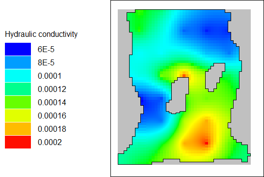
Select File|Import|Gridded Data Files and select the file for the Kx data set in the arrays subdirectory of your model directory. The new data set will be classified under "User Defined|Created from text file." The name of the new data set will be based on the name of the file. A diagram of the estimated distribution of Kx is shown below.

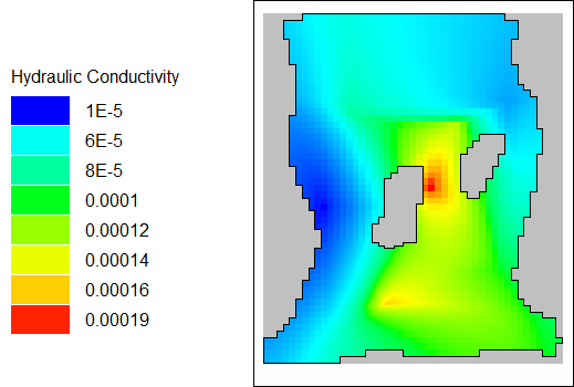
The “true” distribution from the model used to generate the observed values for the parameter estimation exercise is shown below.

Both the estimated and true hydraulic conductivity distributions show patches of low hydraulic conductivity on the west and northeast portions of the model with a higher hydraulic conductivity between the two bedrock islands. The true distribution has more extreme high and low values.