RmaMF6: Define Observations

MODFLOW 6 has an Observation Utility that can generate a times series of simulated values of various types of data generated by the model. ModelMuse can create an input file for Mf6ObsExtractor to cause it to extract simulated values from the time series for use with PEST. For head observations, it will spatially interpolate to the observation location. It will also interpolate in time to the observation time. (Observation times must be relative to the time zero used for the MODFLOW stress periods.) Calibration observations must also have an observed value that will be compared with the simulated value. They must also be assigned a weight. Depending on the observation type various other types of information might be required.

Eight head observation and one flow observation have already been defined in the model as shown in the table below. Now we need to make them calibration observations. We will also define a comparison observation that represents a head gradient between two of the head observations. The head observations are defined by point objects. The flow observation is defined by a polygon object that surrounds part of the object that defines the constant-head boundary near the southern edge of the model. Only those constant head cells whose centers are inside the polygon object are part of the flow observation. The observation values are shown in the table below.  In this example, the observation locations were defined for you. It is also possible to import multiple observations from Shapefiles using the Import Shapefile Dialog Box.

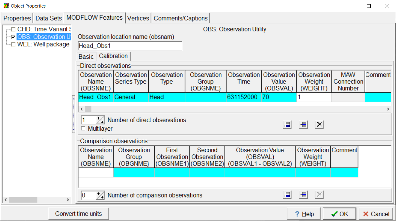
Open each of the objects that defines a head observation one at a time in the Object Properties dialog box and go to the Observation Utility pane on the MODFLOW Features tab. Beneath the Observation location name, select the Calibration tab. In the table for direct observations, enter the observation name, set the series type to General and the Observation type to Head, Leave the observation group (OBGNME) empty for now specify the observation time as 631152000 which is the ending time of the model. Set the observed value according to the table above and set the weight to 1 as illustrated below. Repeat this for each of the head observations. If the model had multiple time steps, we could specify multiple direct observations using different times. We could also specify comparison observations in the table in the lower half of the Calibration tab. For heads, a comparison observation would be the equivalent of a drawdown observation.

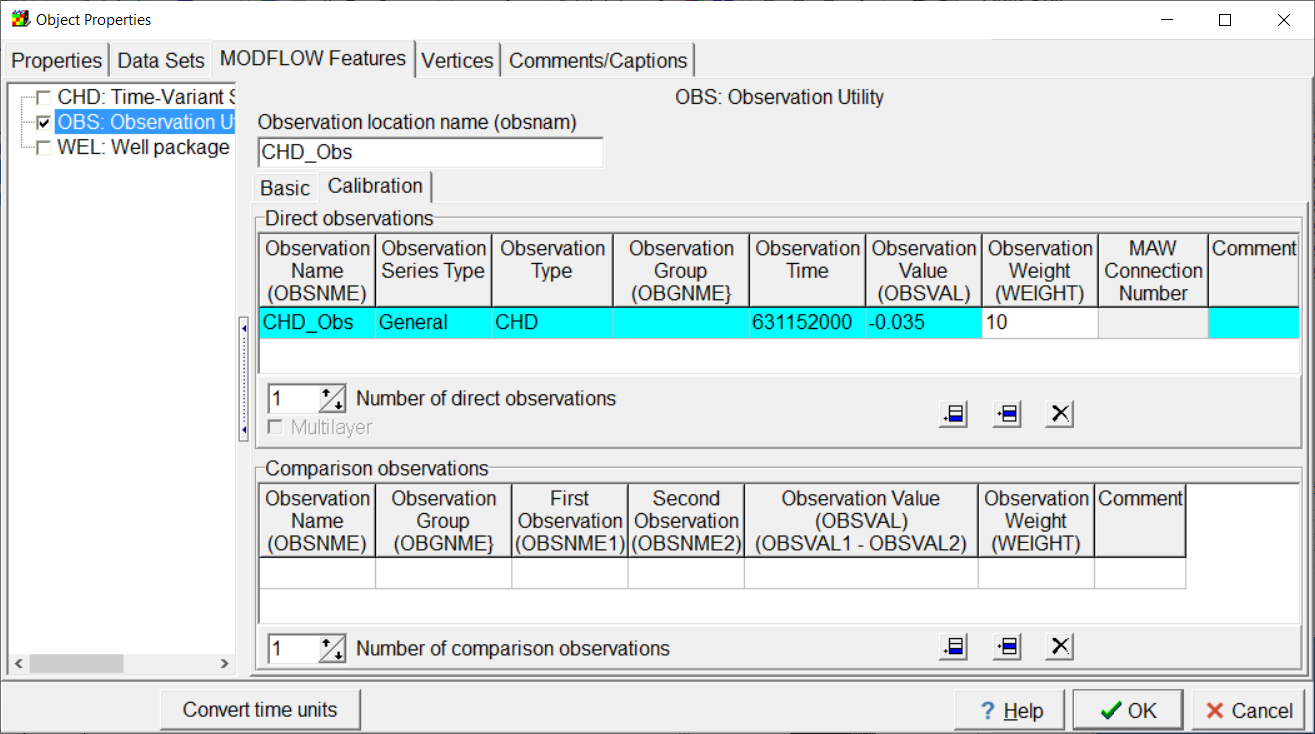
The observation of flow through the southern stream is defined with the object CHD_Obs. It is defined similarly to the head observation. except that the observation type is CHD, and the observation weight is 10 instead of 1 as illustrated below.

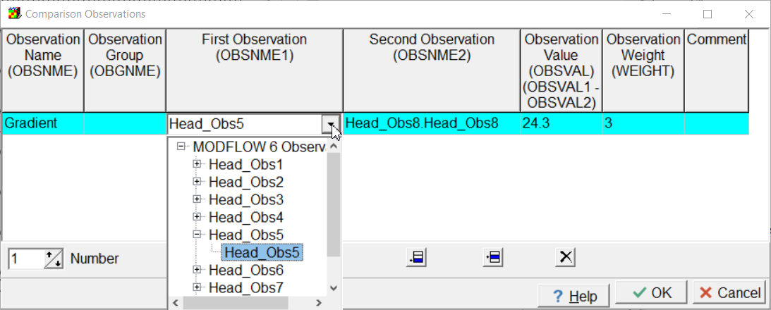
The observed gradient in head between head observations 5 and 8 will also be used as a calibration observation. To add this observation, select Model|Edit Comparison Observations... Specify the observation name, value, and weight (= 3) and select the Head_Obs5 as the first observations and Head_Obs8 as the second observation as illustrated below.