RmaMf2005: Define Observations |
RmaMf2005: Define Observations |
MODFLOW 2005 has observation packages that allow the user to specify observed values, locations, and times head and flow rates. MODFLOW uses these to determine simulated values corresponding to those locations and times. In addition there are several other packages in MODFLOW that report simulated values that could be compared with observed values in the parameter estimation process. ModelMuse can create an input file for Mf2005ObsExtractor to cause it to extract simulated values for use with PEST. For head observations, MODFLOW spatially interpolates to the observation location and will also interpolate in time to the observation time. MODFLOW allows several ways to calculating the weight applied to an observation such as specifying a standard deviation of the observation. When used with PEST, ModelMuse will use appropriate mathematical transformations to convert them to weights.
The locations of eight head observation and one flow observation have already been defined in the model. Now we need to make them observations in MODFLOW-2005 and PEST. We will also define a comparison observation that represents a head gradient between two of the head observations. The head observation locations are defined by unused point objects. The flow observation location is defined by an unused polygon object that surrounds part of the object that defines the constant-head boundary near the southern edge of the model. Only those constant head cells whose centers are inside the polygon object are part of the flow observation. The observation values are shown in the table below. These observed values differ from those in the MODFLOW 6 example model. In this example, the observation locations were defined for you. It is also possible to import multiple observations from Shapefiles using the Import Shapefile Dialog Box.
Observation Name |
Observation Value |
Head_Obs1 |
69.4 |
Head_Obs2 |
63.2 |
Head_Obs3 |
54.6 |
Head_Obs4 |
53.2 |
Head_Obs5 |
50.0 |
Head_Obs6 |
39.0 |
Head_Obs7 |
13.4 |
Head_Obs8 |
27.0 |
CHD_Obs |
-0.037 |
Gradient |
27.0 |
Select Model|MODFLOW Packages and Programs and activate the HOB package under Observations.
The names of the objects that will be used to define head and flow observations will be the same as the observation names. Open each of the objects that will be used to define a head observation in the Object Properties dialog box and go to the HOB: Head Observation Package pane on the MODFLOW Features tab. Specify the observation name, observation time (631152000), observed head from the table above, the Statistic and StatFlag. The Statistic is used to calculate the weight of the observations based on the StatFlag. In the illustrated example, StatFlag represents weight so no conversion is needed.
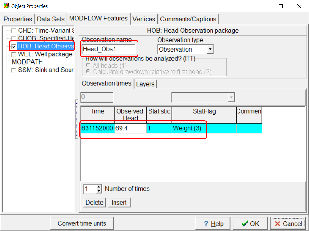
Screen capture illustrating defining a head observation in a MODFLOW-2005 model.
If multiple observations at different times were specified, you could choose to make the second and subsequent observations be calculated as drawdown relative to the first observation with the ITT variable.
Select Model|MODFLOW Packages and Programs and activate the CHOB package under Observations. When you click OK the Manage Flow Observations dialog box will appear.
Flow observations are defined in the Model|Manage Flow Observations dialog box. To define an observation through specified flow boundaries, select CHOB in the list on the left side of the dialog box and then click the Add button. Specify the Observation location name in the edit box on the Observation Properties tab. Specify the observation time (631152000), observed value (-0.037), statistic (10), and StatFlag (Weight) for the observation.
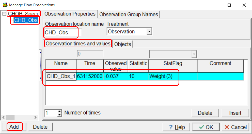
Screen capture illustrating the definition of a flow observation for MODFLOW 2005.
Next switch to the Objects tab and select the Southern_Stream object in the "Available objects" list. Move it to the "Used objects" list by clicking the right arrow button between the two lists.
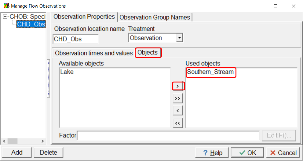
Screen capture illustrating including an object in a flow observation.
We will only include some of the flow through the southern stream as part of the flow observation. We can assign a "Factor' formula to the Southern Stream to accomplish this. Create a new data set named ChobWeight and set its default formula to 0. Then open the unused CHD_Obs object in the Object Properties dialog box. This object surrounds the specified head boundary that we want to include in the flow observation. With the CHD_Obs object, set ChobWeight to 1.
Next open the Southern_Stream object in the in the Object Properties dialog box and set the Factor in the CHD_Obs to ChobWeight. With this change, the flows through the specified head cells defined by the Southern_Stream object will be multiplied by either zero or one depending on whether they are inside or outside the CHD_Obs object. In effect, this excludes the flows through CHD cells outside the CHD_Obs object from the flow observation.
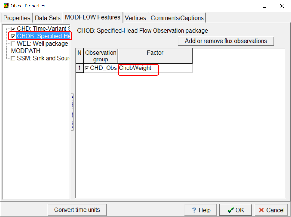
Screen capture illustrating assigning a weight factor to a flow observations.
The observed gradient in head between head observations 5 and 8 will also be used as a calibration observation. To add this observation, select Model|Edit Comparison Observations... Specify the observation name, value and weight and select the Head_Obs5 as the first observations and Head_Obs8 as the second observation. Set the observation weight to 3.
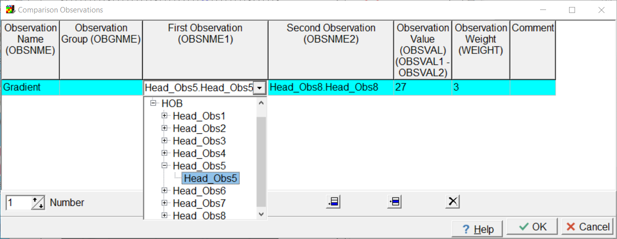
Screen capture illustrating how to specify a comparison observation.