Interpolation Methods

The interpolation method of a data set is used to determine how values should be interpolated among a group of objects. Interpolation can only be used for 2-D data sets. Only one of the PHAST data sets, Initial_Water_Table, is a 2-D data set. All the data sets defining the boundaries between layers in MODFLOW are 2-D data sets. In addition, the user can define his or her own 2-D data sets and use interpolation with them. One appropriate use of such 2-D data sets in PHAST would be to define the tops and bottoms of geologic units.

Eight interpolation algorithms are available in ModelMuse: Nearest, Point Average, Nearest Point, Inv. Dist. Sq. (Inverse Distance Squared), Triangle Interp. (Triangle Interpolation), Fitted Surface, Point Inv. Dist. Sq. (Point Inverse Distance Squared), and Natural Neighbor. If the units of a data set are set to degrees or radians, All of these interpolation methods will be evaluated slightly differently in a way that is more appropriate for angles. See Specifying Angles for SUTRA.

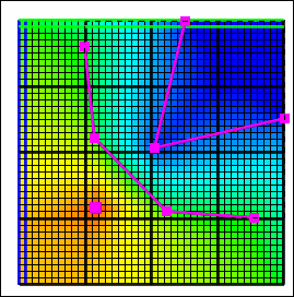
The Nearest interpolation method (fig. 18A) works by determining the object that is closest to the location where the data set in question is being evaluated. Then the formula of that object is evaluated at that location. If all the objects used with the method are point objects, the Nearest Point interpolation method produces the same result more quickly (fig. 19) so the Nearest interpolation method is generally used for line or polygon objects.

The Point Average is only used where there are expected to be enough points so that every cell or element contains at least one point. The value assigned to the element or cell will be the arithmetic average of those points. If no points are in a cell or element, the cell or element will be assigned a value of zero.

The Nearest Point interpolation method (fig. 18B) is similar to the Nearest interpolation method except that only the vertices of objects are considered, rather than the lines connecting the vertices. If only point objects are used, the result is identical. The Nearest Point interpolation method uses an algorithm that is faster (fig. 19) than the Nearest interpolation method when the number of points is greater than several hundred. The Nearest Point interpolation method is the fastest of all the interpolation methods when used with point data (fig. 19). If used with line or polygon data it can be slower than the Nearest interpolation especially if many of the object vertices lie outside the grid.

With the Inv. Dist. Sq. interpolation method (fig. 18C), the formula for each object is evaluated at the location under consideration. The final value is a weighted average of these values. The weights are the inverse of the distance squared from the location to the closest point on each respective object. The Inv. Dist. Sq. interpolation method may only be used with data sets containing real numbers. Because the Inv. Dist. Sq. interpolation method is slow (fig. 19), it generally is not used with more than a few hundred objects. If the formulas for all the objects are numbers and all the objects are point objects, the Point Inv. Dist. Sq. interpolation method gives the same results more quickly (fig. 19).

With the Point Inv. Dist. Sq. interpolation method (fig. 18D), the formula for each vertex for each object is evaluated at its own location. The final value is a weighted average of these values. The weights are the inverse of the distance squared from the location of interest to the vertex. The Point Inv. Dist. Sq. interpolation method may only be used with data sets containing real numbers. If the formulas for all the objects are numbers and all the objects are point objects, the Point Inv. Dist. Sq. interpolation method gives the same results as the Inv. Dist. Sq. interpolation method but does so more quickly (fig. 19).

The Fitted Surface interpolation method (fig. 18E) evaluates the formula for each object at the location of each vertex on the object. It then creates an unconstrained Delaunay triangulation of all the vertices (the same one as in Triangle Interp.). A piece-wise continuous function of the locations is fitted through the data values and the function is used to assign values at each location of interest. This method was created by Renka (1996a, b). The Fitted Surface interpolation method may only be used with data sets containing real numbers. Interpolated values returned by Fitted Surface may be higher than the highest value at any data point or lower than the lowest value at any data point. The Fitted Surface interpolation method is a relatively fast interpolation method (fig. 19).

The Triangle Interp. interpolation method (fig. 18F) evaluates the formula for each object at the location of each vertex on the object. It then creates an unconstrained Delaunay triangulation of all the vertices. If a location where a value is needed is inside one of the triangles, the value assigned to that location will be calculated by fitting a plane to the three points of the triangle and determining the height of the plane at the location of interest. Other locations will be assigned the value that would have been assigned to the closes location on the convex hull of the data points. This method was created by Renka (1996a, b). The Triangle Interp. interpolation method may only be used with data sets containing real numbers. Interpolated values returned by Triangle Interp. are never higher than the highest value at any data point or lower than the lowest value at any data point. The Triangle Interp. interpolation method is a relatively fast interpolation method (fig. 19).

The Natural Neighbor interpolation method (fig. 18G) uses a weighted average of some points near the location of interest. A more detailed description of this method may be found in http://en.wikipedia.org/wiki/Natural_neighbor. Only the vertices of objects are considered, rather than the lines connecting the vertices. The Natural Neighbor method is similar in speed to the Triangle Interp. and Fitted Surface methods (fig. 19) but uses more memory. The Natural Neighbor interpolation method may only be used with data sets containing real numbers. Unlike the Fitted Surface method, interpolated values returned by Natural Neighbor are never higher than the highest value at any data point nor lower than the lowest value at any data point.

A special modification of the interpolation method is used when the units of a data set are set to Degrees or Radians. See Specifying Angles for SUTRA.

 

Figure 18 Interpolation methods. The points and lines are objects with different values. The figures show how the interpolated values vary among interpolation methods when applied to the same data.—(A) Nearest interpolation method, (B) Nearest Point interpolation method, (C) Inv. Dist. Sq. interpolation method, (D) Point Inv. Dist. Sq. interpolation method, (E) Fitted Surface interpolation method, (F) Triangle Interp. interpolation method, and (G) Natural Neighbor interpolation method.