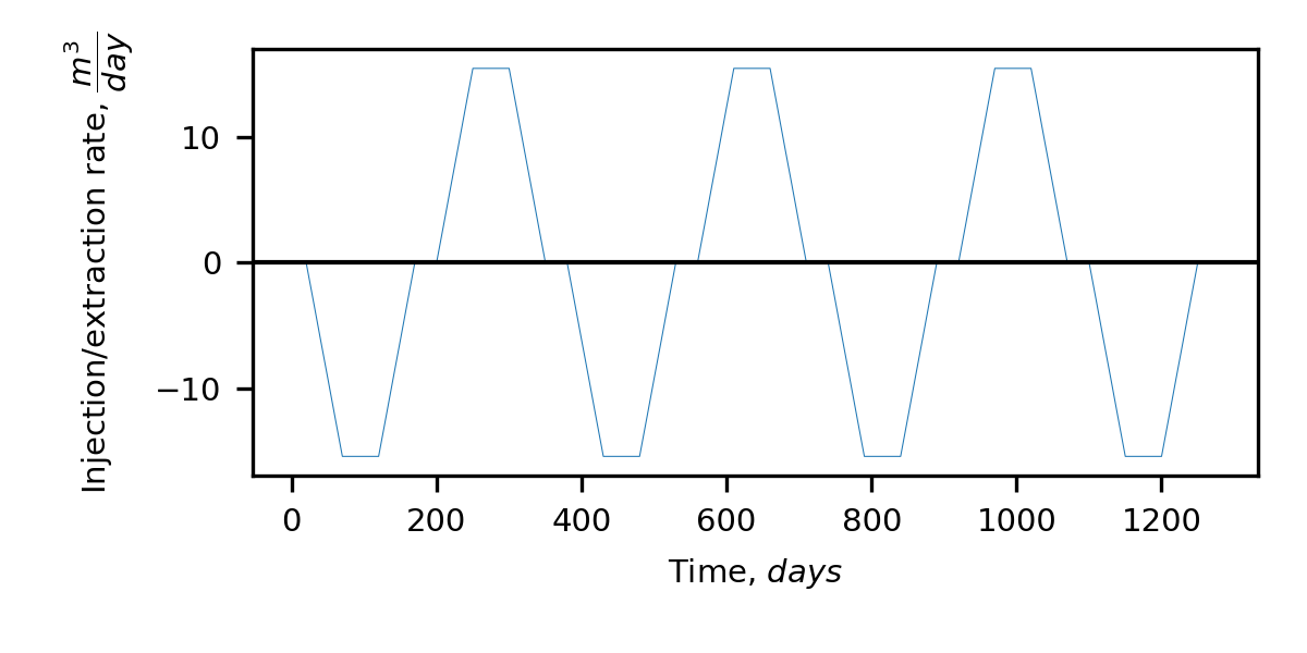
The well extends over cells at the left edge of the model with y-coordinates extending from 15 to 35. The pumping rate varies over time as illustrated below. We will use a time series to define the pumping rates.

A time series of the extraction and injection pumping rates. Negative and positive values indicate extraction and injection, respectively. Pumping occurs on the left side of the model
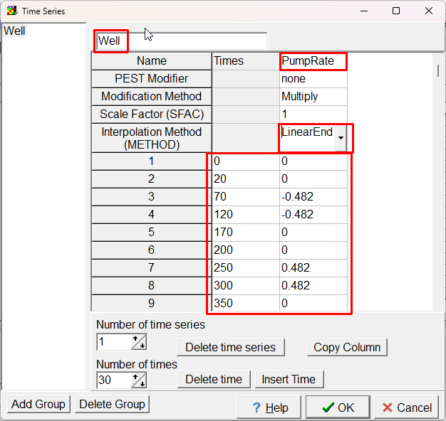
The times and pumping rate can be defined by a time series with the interpolation method set to LinearEnd. Select "Model|Edit Time Series", click "Add Group", define a group name, time series name, and enter the following times and pumping rates. You can copy the block of values to the clipboard and paste it into ModelMuse Be sure to set the interpolation method set to LinearEnd. With "LinearEnd", the applied pumping rate will be applied by interpolating between the specified times to the time at the end of the stress period.
0, 0
20, 0
70, -0.482
120, -0.482
170, 0
200, 0
250, 0.482
300, 0.482
350, 0
380, 0
430, -0.482
480, -0.482
530, 0
560, 0
610, 0.482
660, 0.482
710, 0
740, 0
790, -0.482
840, -0.482
890, 0
920, 0
970, 0.482
1020, 0.482
1070, 0
1100, 0
1150, -0.482
1200, -0.482
1250, 0
1270, 0

Screen capture illustrating the specification of a time series used for seting the pumping rate of the well
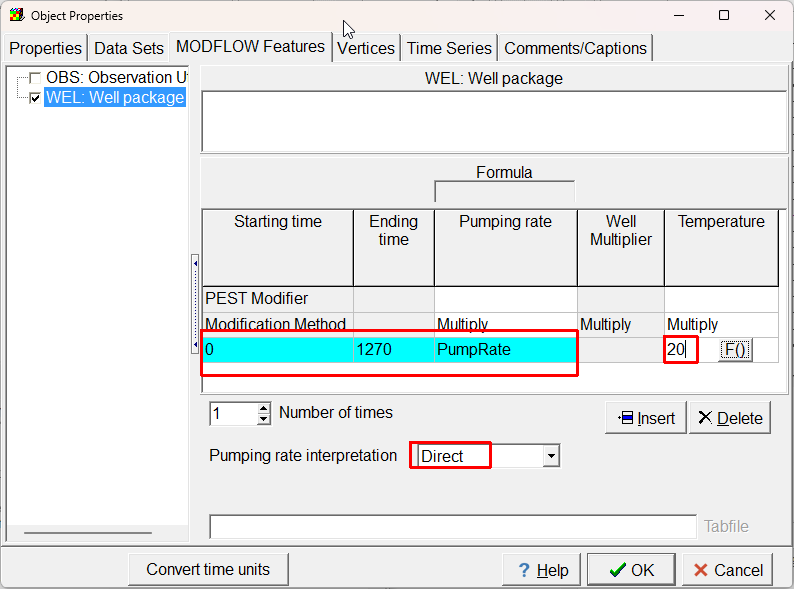
Now create a line object in the first column of cells extending from y = 15 to y = 35. It will be used to define the well. Activate the Well package in the Object Properties dialog box. Set the starting and ending times to encompass the entire model period. Set the pumping rate formula to the name of the time series defined previously and set the associated temperature to 20. This is the temperature of the water when the well is injecting water. When the well is extracting water, the temperature of the extracted water will be the groundwater temperature. Be sure to set the pumping rate interpretation to "Direct."

Screen capture of the Object Properties dialog box specifying the properties of the well