import os
os.environ['USE_PYGEOS'] = '0'
import os.path
from pathlib import Path
# Data objects
import geopandas as gpd
import pandas as pd
import rioxarray as rxr
import xarray as xr

# GDPTools objects
from gdptools import ZonalGen
from gdptools.data.user_data import UserTiffData

# Plotting objects
import matplotlib.pyplot as pltUse Cases
hi-raster-summarization
Keywords: gdptools; zonal statistics; spatial-interpolation
Domain: Hydrology; Topography; Land Use; Land Cover
Language: Python
Description:
This notebook demonstrates the use of gdptools for raster summarization for model parameterization inputs
Raster summarization of select topographic and land use characteristics to the GFv2.0 Hi Fabric
This notebook demonstrates the use of gdptools for raster summarization for model parameterization inputs.
1 Why
Model parameters, such as mean elevation, slope, and land use, can be extracted from rasters for use in hydrologic models. To do this, these parameters must be summarized from a raster to a set of polygons that represent the model’s Hydrologic Response Units (HRUs). For both numerical and categorical raster data, GDPTools offers a collection of tools that interpolate and generate statistics by summarizing the raster pixel values that intersect each HRU in the model domain.
2 Open source python tools
- gdptools: GeoDataProcessing Tools (GDPTools) is a python package for geospatial interpolation - documentation
- Geopandas: Geopandas is a python package for geospatial dataframes.
3 Data
- Configuration file: conda/mamba environment-examples.ymml file https://www.sciencebase.gov/catalog/item/64e3bca3d34e5f6cd554e8f5
- Target geometry: hru polygons from the GIS Features of the Geospatial Fabric for the National Hydrologic Model, Hawaii Domain (Region 20), NHM_20_810.gdp.zip https://www.sciencebase.gov/catalog/file/get/6489dafcd34ef77fcafe5bc2?f=__disk__e7%2F0b%2F93%2Fe70b935ba285fae40d308503ad7f9cc821b5831c
- Source data for Hawaiian Domain: https://www.sciencebase.gov/catalog/item/64e3bca3d34e5f6cd554e8f5
- Topography: dem.zip
- Slope: slope.zip
- Land use land cover: LULC.zip
4 Description
This use case demonstrates processing statistics from three source rasters: a categorical raster (Land-use/Land-cover) and two numeric rasters (Topography and Slope). For each raster, the statistics are calculated using gdptools functions which intersect pixel values for each polygon (hrus from the Geospatial Fabric, Bock et al, 2022) and then summarizes the data for each polygon and saves the results into a csv file. This file can be used with hydrologic models such as the National Hydrologic Model (Regan et al, 2018).
5 References
Regan, R.S., Markstrom, S.L., Hay, L.E., Viger, R.J., Norton, P.A., Driscoll, J.M., LaFontaine, J.H., 2018, Description of the National Hydrologic Model for use with the Precipitation-Runoff Modeling System (PRMS): U.S. Geological Survey Techniques and Methods, book 6, chap B9, 38 p., https://doi.org/10.3133/tm6B9.
Bock, A.R., Blodgett, D.L., Johnson, J.M., Santiago, M., Wieczorek, M.E., 2022, PROVISIONAL: National Hydrologic Geospatial Fabric Reference and Derived Hydrofabrics: U.S. Geological Survey data release, https://doi.org/10.5066/P9NFPB5S
6 Getting started
- Download the data linked in the Data Section above and unzip the dem, LULC and slope files into your working directory.
- Download this notebook.
- Create a conda environment to run the notebook from the environment-examples.yml file (for example: conda env create -f environment-examples.yml).
- Make any adjustments within the notebook to point to the file paths of the source and target datasets if necessary.
- With the conda environment active launch
jupyter notebookorjupyter laband run the noteook.
7 Imports
8 Elevation data
For NHM parameter: hru_elev - Median elevation for each HRU
9 Load source and target data
The user will have to modify the data paths as necessary.
# set some input variables
data_dir = Path.home() / 'data'
output_dir = data_dir / 'results'
if not output_dir.exists():
    os.mkdir(output_dir)
# path to hru dataset
# the_hrus = os.path.join(data_dir, "NHM_20_810.gdb")
the_hrus = data_dir / "NHM_20_810.gdb"
# hrus dataset hru id field name
hru_id = "hru_id"
print(f"the_hrus exists: {the_hrus.exists()}")
# NHM parameter name
param_name = "hru_elev"
# The statistic used to define the parameter value
function = "median"
in_raster = "HI_DataLayersforth/dem/dem.tif"
# dem raster
# the_raster = os.path.join(data_dir, in_raster)
the_raster = data_dir / in_raster
print(f"the_raster exists: {the_raster.exists()}")
the_hrus exists: True
the_raster exists: True10 Read HRUs spatial dataset
hru_id is a field of type integer, with a unique id for each HRU (ranging from one to the number of HRUs)
# Use geopandas to read shape file,
# Best if shape file only has feature id, and geometry if possible.
gdf = gpd.read_file(the_hrus, layer='nhru')
id_feature = hru_id
print(f"Number of features: {len(gdf.groupby(id_feature))}")
# Filter the geodataframe to just the feature id and the geometry columns
gdf = gdf[["hru_id", "geometry"]]
gdf
Number of features: 5649| hru_id | geometry | |
|---|---|---|
| 0 | 1 | MULTIPOLYGON (((905310.000 2183050.000, 905285... |
| 1 | 2 | MULTIPOLYGON (((907007.892 2185180.389, 907034... |
| 2 | 3 | MULTIPOLYGON (((890410.000 2183620.000, 890424... |
| 3 | 4 | MULTIPOLYGON (((891830.978 2184750.282, 891834... |
| 4 | 5 | MULTIPOLYGON (((895710.000 2183440.000, 895670... |
| ... | ... | ... |
| 5644 | 5645 | MULTIPOLYGON (((379720.000 2417440.000, 379527... |
| 5645 | 5646 | MULTIPOLYGON (((377326.970 2424800.293, 377366... |
| 5646 | 5647 | MULTIPOLYGON (((381770.000 2420970.000, 381765... |
| 5647 | 5648 | MULTIPOLYGON (((380940.000 2426340.000, 380944... |
| 5648 | 5649 | MULTIPOLYGON (((384548.178 2428477.734, 384554... |
5649 rows × 2 columns
11 Read raster dataset
# Be sure to use rioxarray to read the tiff
rds_ras = rxr.open_rasterio(the_raster)
12 Look at the raster representation
rds_ras<xarray.DataArray (band: 1, y: 12147, x: 18972)>
[230452884 values with dtype=uint16]
Coordinates:
* band (band) int64 1
* x (x) float64 3.711e+05 3.712e+05 ... 9.402e+05 9.403e+05
* y (y) float64 2.459e+06 2.459e+06 ... 2.094e+06 2.094e+06
spatial_ref int64 0
Attributes:
AREA_OR_POINT: Area
RepresentationType: ATHEMATIC
STATISTICS_MAXIMUM: 4199
STATISTICS_MEAN: 899.49574536833
STATISTICS_MINIMUM: 0
STATISTICS_SKIPFACTORX: 1
STATISTICS_SKIPFACTORY: 1
STATISTICS_STDDEV: 868.55205999837
_FillValue: 65535
scale_factor: 1.0
add_offset: 0.013 Calculate Zonal Statistics
GDPTools provides a data class, UserTiffData(), for parameterizing the source and target input data, and ZonalGen() is used to calculate the statistics of the intersection between source and target data. The parameters for the initialization of the UserTiffData class can largely be read from the raster representaion above. For example ‘x’ is the coordinate name for the x-axis and thus ‘tx_name’ is ‘x’.
# These params are used to fill out the TiffAttributes class
tx_name= 'x'
ty_name = 'y'
band = 1
bname = 'band'
crs = 26904 #
varname = "elev" # not currently used
categorical = False # is the data categorical or not, if the data are integers it should
                   # probably be categorical.
data = UserTiffData(
    var=varname,
    ds=rds_ras,
    proj_ds=crs,
    x_coord=tx_name,
    y_coord=ty_name,
    band=band,
    bname=bname,
    f_feature=gdf,
    id_feature=id_feature,
    proj_feature=crs
)

zonal_gen = ZonalGen(
    user_data=data,
    zonal_engine="serial",
    zonal_writer="csv",
    out_path=".",
    file_prefix="Hi_elev_stats"
)
stats = zonal_gen.calculate_zonal(categorical=categorical)
data prepped for zonal in 0.0102 seconds
converted tiff to points in 12.8243 seconds
- fixing 45 invalid polygons.
overlaps calculated in 11.5290 seconds
zonal stats calculated in 6.0673 seconds
[[ 0]
[2742]]
number of missing values: 1
fill missing values with nearest neighbors in 0.0106 seconds
Total time for serial zonal stats calculation 32.6104 seconds14 Examine the output
stats.head()| count | mean | std | min | 25% | 50% | 75% | max | sum | |
|---|---|---|---|---|---|---|---|---|---|
| hru_id | |||||||||
| 1 | 4269.0 | 167.915203 | 64.230722 | 2.0 | 122.00 | 166.0 | 232.00 | 295.0 | 716830 |
| 2 | 3839.0 | 169.637145 | 73.471249 | 2.0 | 111.00 | 165.0 | 222.00 | 375.0 | 651237 |
| 3 | 3824.0 | 1019.152458 | 53.491336 | 912.0 | 974.00 | 1022.0 | 1058.25 | 1148.0 | 3897239 |
| 4 | 1361.0 | 996.487877 | 65.453340 | 911.0 | 945.00 | 967.0 | 1043.00 | 1151.0 | 1356220 |
| 5 | 764.0 | 854.184555 | 37.486651 | 760.0 | 823.75 | 862.5 | 881.25 | 914.0 | 652597 |
15 Define function to generate NHM parameter files
A NHM parameter file is a csv file consisting of two columns. The first column named $id contains the hru_id (in sequential order starting with 1). The second column contains the corresponding parameter value for the HRU, and the colunm name is the parameter name, for example, hru_elev.
# Function to output results to NHM parameter file format
def stats_to_paramcsv2(param_name, stats, categorical, function, hru, hru_id, output_dir):
    # purpose: to write result of gdptools to parameter file
    #          and to add param to hru geopandas df for plots
    # arguments:
    #   param_name - character - specifying the ParamDB parameter name,
    #      for example:  hru_slope  hru_elev
    #   stats - pandas df, output from gdptools function
    #          (cols like a pandas describe)
    #   categorical - Boolean (it determines the stats field names)
    #   function - chararacter -(function valid values for categorical False: sum, mean, median min, max)
    #                      function for categorical True is majority (or top)
    #   hru - geopandas df
    #   hru_id - character - hru id field name
    #    output_dir - character - parameter file output path
    outpth = os.path.join(output_dir, '%s.csv'%(param_name))
    #outpth = output_dir / (param_name + '.csv')
    if(categorical):
        thepar_df = stats[['top']].rename(columns = {'top':param_name})
        hru[param_name] = stats['top'].values
        # rename the id field parameter file
        thepar_df.index.name = "$id"
        thepar_df.to_csv(outpth, index = True)
    else:
        stats.rename(columns = {'50%':'median'}, inplace = True)
        function_list = ["mean", "min","max", "sum","median"]
        if (function in function_list):
            # for slope div 100
            if param_name == "hru_slope":
                thepar_df = stats[[function]].rename(columns = {function:param_name})
                thepar_df[param_name] = thepar_df[param_name] / 100
                hru[param_name] = stats[function].values / 100
            else :
                thepar_df = stats[[function]].rename(columns = {function:param_name})
                hru[param_name] = stats[function].values
            thepar_df.index.name = "$id"
            thepar_df.to_csv(outpth, index = True)
        else:
            print("ERROR: invalid function: {0}".format(function))
            print("No param file generated")
            thepar_df = pd.DataFrame()
    return(thepar_df)
16 Define plotting function
def vis_the_map(the_df,param_name,the_cmap):
# histogram
    plt.hist(the_df[param_name], edgecolor = 'black')
    plt.xlabel(param_name)
    plt.ylabel('value count')
    plt.show()
    # map
    hru.plot(param_name, cmap = the_cmap, legend = True)
    plt.title(param_name)
    plt.show()
    return
17 Generate parameter file for hru_elev
hru = gdf.copy()
tst_df = stats_to_paramcsv2(param_name, stats, categorical, function, hru, hru_id, output_dir)
18 Examine the output
tst_df.head()| hru_elev | |
|---|---|
| $id | |
| 1 | 166.0 |
| 2 | 165.0 |
| 3 | 1022.0 |
| 4 | 967.0 |
| 5 | 862.5 |
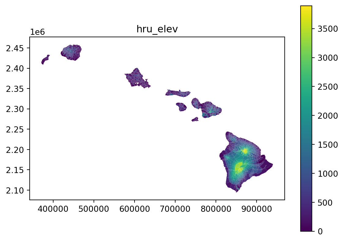
19 Visualize the results as a histogram and map plot
vis_the_map(tst_df,param_name,'viridis')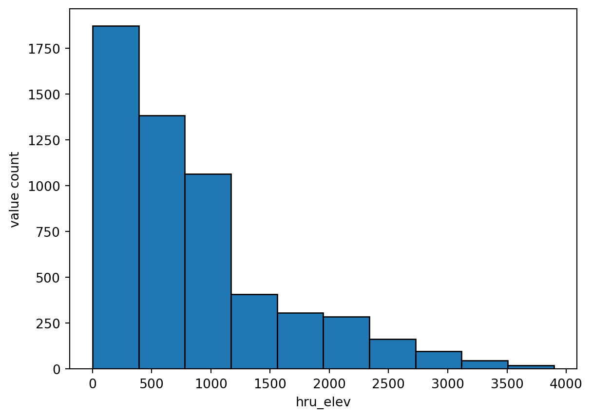
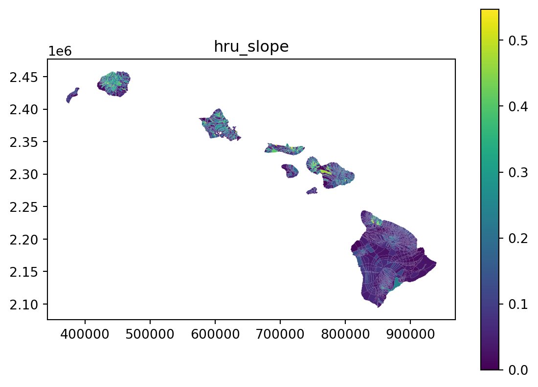
20 Repeat the steps above for the slope parameter
For NHM parameter hru_slope - Mean slope for each hru
param_name = "hru_slope"
function = "mean"
in_raster = "HI_DataLayersforth/slope/slope.tif"
# dem raster
# the_raster = os.path.join(data_dir, in_raster)
the_raster = data_dir / in_raster
print(f"the_raster exists: {the_raster.exists()}")
the_raster exists: True21 Read raster dataset
# use rioxarray to read the tiff
rds_ras = rxr.open_rasterio(the_raster)
rds_ras
<xarray.DataArray (band: 1, y: 12147, x: 18972)>
[230452884 values with dtype=int32]
Coordinates:
* band (band) int64 1
* x (x) float64 3.711e+05 3.712e+05 ... 9.402e+05 9.403e+05
* y (y) float64 2.459e+06 2.459e+06 ... 2.094e+06 2.094e+06
spatial_ref int64 0
Attributes:
AREA_OR_POINT: Area
RepresentationType: ATHEMATIC
STATISTICS_MAXIMUM: 79
STATISTICS_MEAN: 8.7074260287955
STATISTICS_MINIMUM: 0
STATISTICS_SKIPFACTORX: 1
STATISTICS_SKIPFACTORY: 1
STATISTICS_STDDEV: 10.006163665482
_FillValue: -2147483648
scale_factor: 1.0
add_offset: 0.022 Calculate Zonal Statistics
# These params are used to fill out the TiffAttributes class
tx_name= 'x'
ty_name = 'y'
band = 'band'
crs = 26904
varname = "slope" # not currently used
categorical = False # is the data categorical or not, if the data are integers it should
                   # probably be categorical.
data = UserTiffData(
    var=varname,
    ds=rds_ras,
    proj_ds=crs,
    x_coord=tx_name,
    y_coord=ty_name,
    band=1,
    bname=band,
    f_feature=gdf,
    id_feature=id_feature,
    proj_feature=crs
)

zonal_gen = ZonalGen(
    user_data=data,
    zonal_engine="serial",
    zonal_writer="csv",
    out_path=".",
    file_prefix="Hi_slope_stats"
)
stats = zonal_gen.calculate_zonal(categorical=categorical)
data prepped for zonal in 0.0115 seconds
converted tiff to points in 10.7371 seconds
- fixing 45 invalid polygons.
overlaps calculated in 12.9599 seconds
zonal stats calculated in 5.8384 seconds
[[ 0 1 2]
[ 571 2741 3316]]
number of missing values: 3
fill missing values with nearest neighbors in 0.0115 seconds
Total time for serial zonal stats calculation 32.0670 secondsstats.head()| count | mean | std | min | 25% | 50% | 75% | max | sum | |
|---|---|---|---|---|---|---|---|---|---|
| hru_id | |||||||||
| 1 | 4269.0 | 4.224877 | 3.848773 | 0.0 | 2.0 | 3.0 | 5.0 | 31.0 | 18036 |
| 2 | 3839.0 | 5.544934 | 4.178844 | 0.0 | 3.0 | 4.0 | 6.0 | 29.0 | 21287 |
| 3 | 3824.0 | 3.458159 | 1.544637 | 0.0 | 2.0 | 3.0 | 4.0 | 12.0 | 13224 |
| 4 | 1361.0 | 3.686260 | 2.203112 | 0.0 | 2.0 | 3.0 | 5.0 | 12.0 | 5017 |
| 5 | 764.0 | 3.833770 | 2.033755 | 0.0 | 2.0 | 4.0 | 5.0 | 12.0 | 2929 |
23 Create slope parameter file
hru = gdf.copy()
# generate parameter file
tst_df = stats_to_paramcsv2(param_name, stats, categorical, function, hru, hru_id, output_dir)
tst_df.head()| hru_slope | |
|---|---|
| $id | |
| 1 | 0.042249 |
| 2 | 0.055449 |
| 3 | 0.034582 |
| 4 | 0.036863 |
| 5 | 0.038338 |
24 Visualize the results
vis_the_map(tst_df,param_name,'viridis')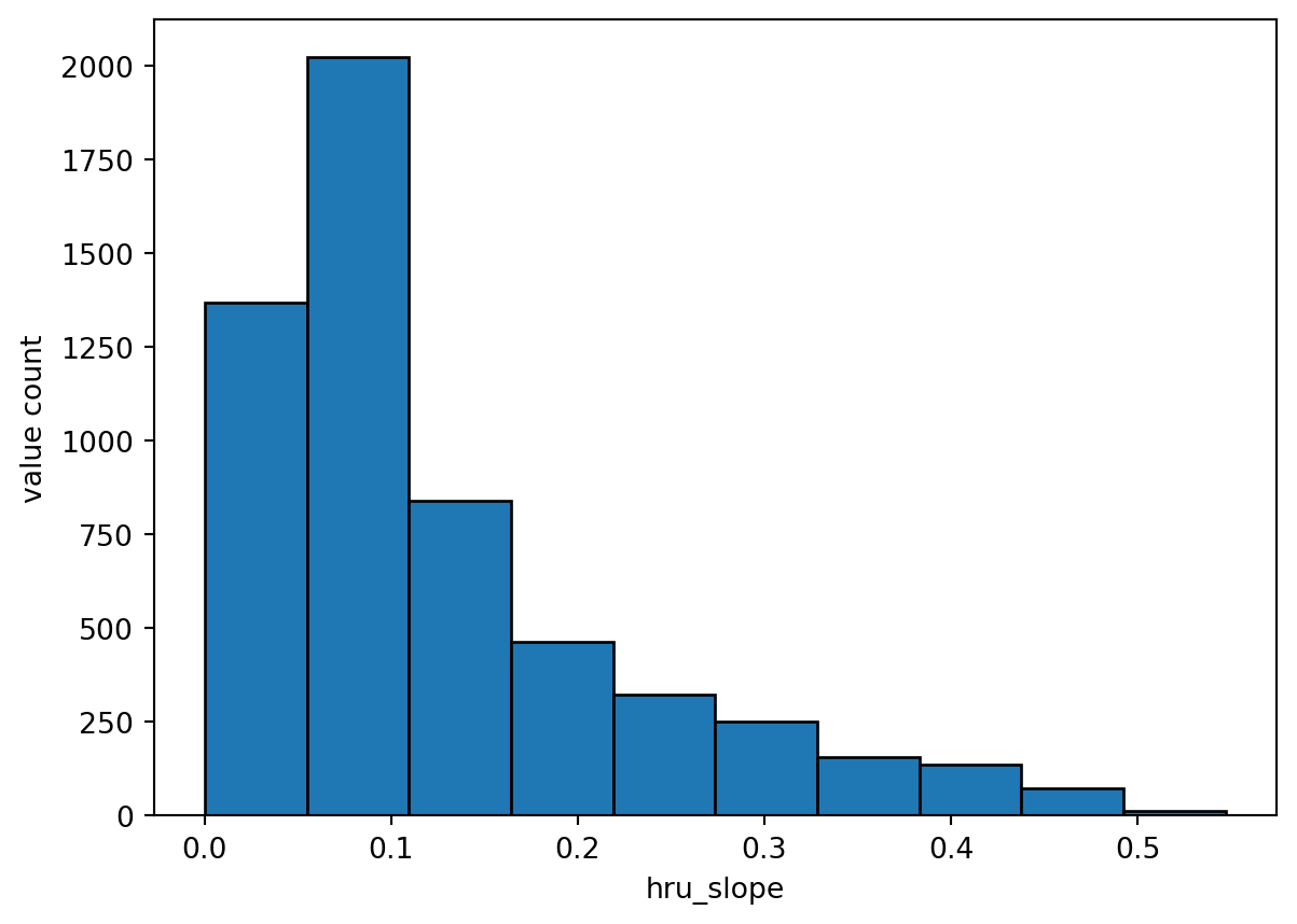
25 Repeat the process for a categorical data - Land Use Land Cover
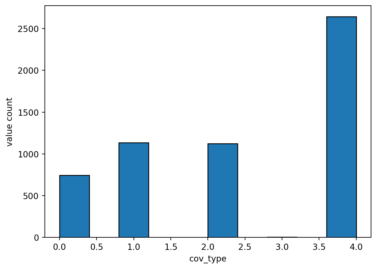
For NHM cov_type parameter file - Vegetation cover type for each hydrologic response unit (0=bare soil; 1=grasses; 2=shrubs; 3=trees; 4=coniferous)
param_name = "cov_type"
function = "top"
in_raster = "HI_DataLayersforth/LULC/LULC.tif"
# dem raster
# the_raster = os.path.join(data_dir, in_raster)
the_raster = data_dir / in_raster
print(f"the_raster exists: {the_raster.exists()}")
the_raster exists: True26 Read raster dataset
# use rioxarray to read the tiff
rds_ras = rxr.open_rasterio(the_raster)
rds_ras
<xarray.DataArray (band: 1, y: 12148, x: 18973)>
[230484004 values with dtype=int8]
Coordinates:
* band (band) int64 1
* x (x) float64 3.711e+05 3.711e+05 ... 9.402e+05 9.403e+05
* y (y) float64 2.459e+06 2.459e+06 ... 2.094e+06 2.094e+06
spatial_ref int64 0
Attributes:
AREA_OR_POINT: Area
RepresentationType: ATHEMATIC
STATISTICS_MAXIMUM: 4
STATISTICS_MEAN: 1.9124980652607
STATISTICS_MINIMUM: 0
STATISTICS_SKIPFACTORX: 1
STATISTICS_SKIPFACTORY: 1
STATISTICS_STDDEV: 1.4947221307764
_FillValue: -128
scale_factor: 1.0
add_offset: 0.027 Calculate Zonal Statistics
# These params are used to fill out the TiffAttributes class
tx_name= 'x'
ty_name = 'y'
band = 'band'
crs = 26904
varname = "LULC" # not currently used
categorical = True # is the data categorical or not, if the data are integers it should
                   # probably be categorical.
data = UserTiffData(
    var=varname,
    ds=rds_ras,
    proj_ds=crs,
    x_coord=tx_name,
    y_coord=ty_name,
    band=1,
    bname=band,
    f_feature=gdf,
    id_feature=id_feature,
    proj_feature=crs
)

zonal_gen = ZonalGen(
    user_data=data,
    zonal_engine="serial",
    zonal_writer="csv",
    out_path=".",
    file_prefix="Hi_cov_type_stats"
)
stats = zonal_gen.calculate_zonal(categorical=categorical)
data prepped for zonal in 0.0187 seconds
converted tiff to points in 10.1269 seconds
- fixing 45 invalid polygons.
overlaps calculated in 12.5668 seconds
categorical zonal stats calculated in 4.1942 seconds
[[ 0]
[2742]]
number of missing values: 1
fill missing values with nearest neighbors in 0.0087 seconds
Total time for serial zonal stats calculation 31.1779 seconds28 View the categorical statistics
stats| count | unique | top | freq | |
|---|---|---|---|---|
| hru_id | ||||
| 1 | 4269 | 4 | 0 | 2029 |
| 2 | 3839 | 5 | 1 | 2414 |
| 3 | 3824 | 3 | 4 | 3696 |
| 4 | 1361 | 2 | 4 | 1352 |
| 5 | 764 | 2 | 4 | 720 |
| ... | ... | ... | ... | ... |
| 5646 | 10044 | 4 | 2 | 7131 |
| 5647 | 38745 | 5 | 2 | 29073 |
| 5648 | 5750 | 4 | 2 | 5070 |
| 5649 | 16864 | 5 | 2 | 15789 |
| 2335 | 70 | 1 | 4 | 70 |
5649 rows × 4 columns
29 Create cov_type parameter file
hru = gdf.copy()
# generate parameter file
tst_df = stats_to_paramcsv2(param_name, stats, categorical, function, hru, hru_id, output_dir)
tst_df.head()| cov_type | |
|---|---|
| $id | |
| 1 | 0 |
| 2 | 1 |
| 3 | 4 |
| 4 | 4 |
| 5 | 4 |
30 Visualize the results
vis_the_map(tst_df,param_name,'viridis')