Description:

Overview of accessing spatio-temporal data via the OGC EDR API via a deployed pygeoapi instance.

Environmental Data Retrieval (EDR) Use Case

Introduction

The Open Geospatial Consortium (OGC) Environmental Data Retrieval (EDR) API provides a family of lightweight query interfaces to access spatio-temporal data resources stored in Zarr or netCDF formats. pygeoapi is a Python server implementation of the OGC suite of standards that inclues an EDR provider, allowing the USGS to serve spatio-temporal data in cloud storage (e.g. on the Open Storage Network or AWS S3 ) in alignment with the OGC API standard. This use case demonstrates how users can access data stored in a Zarr file on USGS’s Open Storage Network (OSN) pod using the OGC EDR API via their deployed pygeoapi instance.

The USGS Geo Data Portal Server is a deployed pygeoapi instance that contains EDR endpoints. Currently, only a few of the possible queries have been implemented by the pygeoapi EDR provider including: position and cube. However there are many other possible queries that we indend to develop in the future. Visit the demo EDR SwaggerUI for full set of query endpoints.

Open Source Python Tools

• pygeoapi
  • Key open source dependencies include xarray to read and manipulate multidimensional arrays and fsspec to access cloud storage.

Data

This use case will demonstrate how to access Parameter-elevation Regressions on Independent Slopes Model ( PRISM ) data. This is monthly precipitation, minimum temperature, and maximum temperature from the continental United States (CONUS) between January 1895 to December 2020. PRISM is stored as a Zarr file on the USGS OSN pod.

Use Case Examples

The data can be accessed via the RESTful OGC EDR API; this use case will demonstrate how to access PRISM programatically rogramatically with Python’s requests library.

Programatic Request

Setting Up

Start by importing the requests library, along with some shapely geometries.

import requests
from shapely.geometry import Point

Getting Oriented

Users can start by accessing information about this dataset to understand the spatio-temporal extents and parameters before querying the data. To make a request, define the base URL for the PRISM collection as follows:

URL_ROOT = 'https://api.water.usgs.gov/gdp/pygeoapi'
COLLECTION_NAME = 'PRISM'

collection_request_url = f'{URL_ROOT}/collections/{COLLECTION_NAME}'

Then, run a get request to access metadata about the PRISM dataset in json format:

prism_info= requests.get(
    collection_request_url,
    params={
        'f': 'json',
        'lang': 'en-US',
    }
)

The following commands can provide key information about the dataset:

import pprint
pp = pprint.PrettyPrinter(indent=1, width=80)

pp.pprint(prism_info.json()['parameter_names'])
pp.pprint(prism_info.json()['extent'])

In the case of PRISM, this reveals that the dataset includes 3 variables: ppt (monthly precipitation in mm), tmn (minimum monthly temperature in degrees Celsius), and tmx (maximum monthly temperature in degrees Celcius). These commands show that the data covers CONUS from 1895 to 2020.

Querying the Data

Position Query

Now that the spatio-temporal extents and variables are understood, run a position query to request data in a specific place over time. To set up a position query, update the request URL as follows:

EDR_QUERY = 'position'

request_url = f'{URL_ROOT}/collections/{COLLECTION_NAME}/{EDR_QUERY}'

Note: pygeoapi currently also offers a cube query, shown in the Cube Query section. The OGC EDR Standard contains a full list of queries that should offered with an OGC EDR API; however, pygeoapi does not currently support the remaining queries.

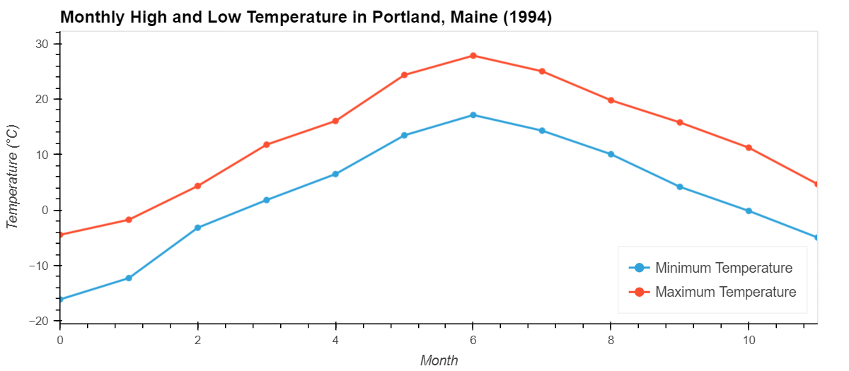
Next, run a get request to get a timeseries of minimum and maximum temperature values at a single point over one year:

prism_subset = requests.get(
    request_url,
    params={
        'coords': Point(-70.31, 43.68),
        'parameter-name': 'tmn,tmx',
        'datetime': '1994-01-01/1994-12-31'
    }
)

The response can be accessed like so:

pp.pprint(prism_subset.json())

Read the Results of the Request

The result is returned as a CoverageJson , a format for spatio-temporal data. The code below reads the CoverageJson response returned by the request.

import geopandas as gpd
import pandas as pd
import numpy as np
from pandas.tseries.offsets import MonthBegin
coverage_dict = prism_subset.json()

# Extract spatial data
x_start, x_stop, x_num = coverage_dict['domain']['axes']['x'].values()
x_values = np.linspace(x_start, x_stop, x_num)

y_start, y_stop, y_num = coverage_dict['domain']['axes']['y'].values()
y_values = np.linspace(y_start, y_stop, y_num)

# Extract Temperature values
tmx_values = coverage_dict['ranges']['tmx']['values']
tmn_values = coverage_dict['ranges']['tmn']['values']

# Extract time data and generate time points
# Initialize list and start date
t_values = []
time_info = coverage_dict['domain']['axes']['time']
current_date = pd.Timestamp(time_info['start'])

# Generate time steps
for _ in range(time_info['num']):
    t_values.append(current_date)
    current_date += MonthBegin(1)  # or MonthEnd(1) depending on your specific case

t_values = [str(t) for t in t_values]

# Create DataFrame
records = []
index = 0
for t in t_values:
    for x in x_values:
        for y in y_values:
            if index < len(tmx_values):
                tmax = tmx_values[index]
                tmin = tmn_values[index]
                records.append({'x': x, 'y': y, 'time': t, 'tmax': tmax, 'tmin': tmin})
                index += 1

df = pd.DataFrame.from_records(records)

# Convert time column to datetime type
df['time'] = pd.to_datetime(df['time'])

# Convert DataFrame to GeoDataFrame
gdf = gpd.GeoDataFrame(df, geometry=gpd.points_from_xy(df.x, df.y))

# Show GeoDataFrame
print(gdf)

This solution allows us to visualize the results. The code below demonstrates quick plotting solutions using Matplotlib and Holoviews.

# Matplotlib
df.plot(x='time', y=['tmax', 'tmin'], xlabel="Month", ylabel="Temperature")

# Holoviews
figure = hv.Curve(df[['time', 'tmax']], label = 'Maximum Temperature') * \
hv.Curve(df[['time', 'tmin']], label = 'Minimum Temperature') * \
hv.Scatter(df[['time', 'tmax']], label = 'Maximum Temperature').opts(size=5) * \
hv.Scatter(df[['time', 'tmin']], label = 'Minimum Temperature').opts(size=5)

figure.opts(legend_position='bottom_right',
    xlabel='Month',
    ylabel='Temperature (°C)',
    title='Monthly High and Low Temperature in Portland, Maine (1994)',
    height=350,
    width=700,
    )

Additional Notes on Querying

• Users can query a single parameter at a time (e.g., replace 'tmn,tmx' above with just 'tmn') up to as many parameters exist in the dataset (e.g., 'tmn,tmx,ppt').
• Users can also query a single datetime by replacing the range above with a single date, rather than a range of dates separated by a forward slash (e.g. '1994-01-01').
• Users can also replace a date on either side of the date range with '..' to query up to the start or end of the dataset.
  • '1994-01-01/..' would retrieve all data from 1994 to the end of the date range in the dataset.
  • '../1994-01-01' would retrieve all data up until 1994.
  • You can even query '../..' to get all of the dates; however, this same result could be achieved by not adding the datetime parameter to your request.

Cube Query

The cube query returns data over a bounding box rather than a single point. To define the request URL for the cube query, update the EDR_QUERY to be 'cube'. Use the bbox query parameter (rather than the coords parameter used for the position query) to define the bounding box over which you would like to retrieve data.

EDR_QUERY = 'cube'

request_url = f'{URL_ROOT}/collections/{COLLECTION_NAME}/{EDR_QUERY}'

prism_cube_subset = requests.get(
    request_url,
    params={
        'bbox': '-100,-98,40,42',
        'parameter-name': 'tmn,tmx',
        'datetime': '1994-01-01/1994-12-31'
    }
)

This result is also returned as a CoverageJson.