from osgeo import gdal
import geopandas as gpd
import pandas as pd
import hvplot.pandas
import hvplot.xarray
import warnings
import xarray as xr

from gdptools import InterpGen
from gdptools import ClimRCatData

warnings.filterwarnings("ignore")Use Cases
Aggregate gridMET data to NHD Flowlines and sample points
Keywords: hydrology; geospatial
Domain: Domain Agnostic
Language: Python
Description:
Using the gdptools python package, aggregate gridMET climate data to a NHD Flowline and return the aggregated values at regularly space sample points.
Linked Catalog Datasets:
Linked Catalog Tools:
GridMET Grid-to-line intersection
Introduction
In this example, the ClimateR-catalog (CRC) developed by Mike Johnson is used to discover a gridded dataset of interest. The CRC encompasses a wealth of data sources and the metadata required to simplify the process of grid-to-polygon area weighted intersections. The CRC here uses a json catalog schema with common metadata for geospatial analysis. In the example below, we aggregate gridMET Daily Maximum Temperature, Daily Minimum Temperature and Daily Precipitation data to several National Hydrology Dataset (NHD) flowlines in HUC 0708.
Geo Data Processing Tools (gdptools)
gdptools is a python package for calculating area-weighted statistics of grid-to-polygon. grid-to-line, and polygon-to-polygon interpolations. gdptools utilizes metadata from the CLimateR Catalog to aid generalizing gdptools processing capabilities. There are also methods for calculating area-weighted statistics for any gridded dataset that can be opened by xarray, however some of the metadata encapsulated in the json entries will have to be added by the user. Examples can be found in Non-Catalog Examples.
Open Source Python Tools
- xarray: Package to work with labelled multi-dimensional arrays.
- geopandas: Package to work with geospatial data.
Data
- gridMET: A dataset of daily high-spatial resolution (~4-km, 1/24th degree) surface meteorological data covering the contiguous US from 1979-yesterday.
- NHDPlus_V2: National Hydrography Dataset Plus Version 2, a selection of flowline geometries from HUC 0708
Maintenance Schedule
- The intent of this notebook is simply a demonstration of an application or workflow. As we progress in the build-out of NGHF project tools, this notebook may be updated or replaced. There is no other planned maintenance at this time.
Description

This workflow demonstrates the grid to line interpoltion functionality from the gdptools package. The purpose of this tool is to attribute gridded data to line geometries. This is done by interpolating points along each line geometry and extracting the underlaying gridded data values at those points. From this point values, statistics are calculated and attributed to the original input lines.
The inputs to the line interpolation tool are a Geopandas geodataframe containing the line geometries, and a Pandas dataframe containing information about the gridMET gridded data. The line interpolation tool can process multi-dimensional xarray data, outputing the statistics organized by each time segment. Also, multiple gridded datasets can be processed, so for the gridMET example, three different climate variables will be accessed and processed.
The outputs are a dataframe containing the statistics for each line geometries calculated for each gridded dataset at each time segment, as well as a geodataframe containing the interpolated point geometries which have the linearly interpolated values from the gridded dataset. Depending on the user’s inputs, the sample points can be interpolated from the line geometry at regular intervals, or the line vertices can be used instead.
Requirements
- Linux OS or Windows OS
- Conda-based package manager such as miniconda or mamba
- A copy of the NHDFlowline.shp file which can be retrieved from the sciencebase link above under Data
Create conda environment
cd to folder containing the environment.yml
cd gdptools # create conda environment conda env create -f gdptools-examples.yml # activate conda environment conda activate gdptools-examples # cd into the folder containing the notebook cd docs/Examples # run jupyter notebook jupyter notebook
Get lines to query data
Open a lines shapefile as a geodataframe. Use these vector geometries to access underlaying gridded data values and calculate statistics for.
# Open line shapefile
gdf = gpd.read_file('./test_lines/test_lines.shp')

# Select just a few flowlines
gdf = gdf[(gdf.permanent_ == '155843758') | (gdf.permanent_ == '155843335') | (gdf.permanent_ == '155842105')]
Get gridded data
Access the climateR-catalog. Use it to make queries for specific gridded dataset in order to coolect the metadata needed to access the gridded datasets.
climater_cat = "https://mikejohnson51.github.io/climateR-catalogs/catalog.parquet"
cat = pd.read_parquet(climater_cat)
cat.head()| id | asset | URL | type | varname | variable | description | units | model | ensemble | ... | Xn | Y1 | Yn | resX | resY | ncols | nrows | crs | toptobottom | tiled | |
|---|---|---|---|---|---|---|---|---|---|---|---|---|---|---|---|---|---|---|---|---|---|
| 0 | maca_day | agg_macav2metdata_huss_BNU-ESM_r1i1p1_historic... | http://thredds.northwestknowledge.net:8080/thr... | opendap | specific_humidity | huss | Daily Mean Near-Surface Specific Humidity | kg kg-1 | BNU-ESM | r1i1p1 | ... | -67.064758 | 25.063078 | 49.396023 | 0.041666 | 0.041666 | 1386.0 | 585.0 | +proj=longlat +a=6378137 +f=0.0033528106647474... | True | T |
| 1 | maca_day | agg_macav2metdata_huss_CNRM-CM5_r1i1p1_histori... | http://thredds.northwestknowledge.net:8080/thr... | opendap | specific_humidity | huss | Daily Mean Near-Surface Specific Humidity | kg kg-1 | CNRM-CM5 | r1i1p1 | ... | -67.064758 | 25.063078 | 49.396023 | 0.041666 | 0.041666 | 1386.0 | 585.0 | +proj=longlat +a=6378137 +f=0.0033528106647474... | True | T |
| 2 | maca_day | agg_macav2metdata_huss_CSIRO-Mk3-6-0_r1i1p1_hi... | http://thredds.northwestknowledge.net:8080/thr... | opendap | specific_humidity | huss | Daily Mean Near-Surface Specific Humidity | kg kg-1 | CSIRO-Mk3-6-0 | r1i1p1 | ... | -67.064758 | 25.063078 | 49.396023 | 0.041666 | 0.041666 | 1386.0 | 585.0 | +proj=longlat +a=6378137 +f=0.0033528106647474... | True | T |
| 3 | maca_day | agg_macav2metdata_huss_bcc-csm1-1_r1i1p1_histo... | http://thredds.northwestknowledge.net:8080/thr... | opendap | specific_humidity | huss | Daily Mean Near-Surface Specific Humidity | kg kg-1 | bcc-csm1-1 | r1i1p1 | ... | -67.064758 | 25.063078 | 49.396023 | 0.041666 | 0.041666 | 1386.0 | 585.0 | +proj=longlat +a=6378137 +f=0.0033528106647474... | True | T |
| 4 | maca_day | agg_macav2metdata_huss_CanESM2_r1i1p1_historic... | http://thredds.northwestknowledge.net:8080/thr... | opendap | specific_humidity | huss | Daily Mean Near-Surface Specific Humidity | kg kg-1 | CanESM2 | r1i1p1 | ... | -67.064758 | 25.063078 | 49.396023 | 0.041666 | 0.041666 | 1386.0 | 585.0 | +proj=longlat +a=6378137 +f=0.0033528106647474... | True | T |
5 rows × 28 columns
Query the climateR-catalog for precipitation and temperature datasets (“tmmn”, “tmmx”, “pr”). Use this gridded data for extract values to assign attirbutes to the overlaying vector geometries.
# Create a dictionary of parameter dataframes for each variable
_id = "gridmet"
tvars = ["tmmn", "tmmx", "pr"]
cat_params = [
    cat.query(
        "id == @_id & variable == @_var"
    ).to_dict(orient="records")[0] for _var in tvars
]

cat_dict = dict(zip(tvars, cat_params))

# Output an example of the cat_param.json entry for "tmmn".
cat_dict.get("tmmn")
{'id': 'gridmet',
'asset': 'agg_met_tmmn_1979_CurrentYear_CONUS',
'URL': 'http://thredds.northwestknowledge.net:8080/thredds/dodsC/agg_met_tmmn_1979_CurrentYear_CONUS.nc',
'type': 'opendap',
'varname': 'daily_minimum_temperature',
'variable': 'tmmn',
'description': 'tmmn',
'units': 'K',
'model': None,
'ensemble': None,
'scenario': None,
'T_name': 'day',
'duration': '1979-01-01/..',
'interval': '1 days',
'nT': nan,
'X_name': 'lon',
'Y_name': 'lat',
'X1': -124.76666663333334,
'Xn': -67.05833330000002,
'Y1': 49.400000000000006,
'Yn': 25.066666666666666,
'resX': 0.041666666666666664,
'resY': 0.04166666666666668,
'ncols': 1386.0,
'nrows': 585.0,
'crs': '+proj=longlat +a=6378137 +f=0.00335281066474748 +pm=0 +no_defs',
'toptobottom': False,
'tiled': ''}Initiate an ClimRCatData object
The ClimRCatData class takes the dataframes created above, which contain all the necessary information for accessing and processing the gridded datasets. The data class required a unique id number for each polygon in the geodataframe (“id_feature”) and the time period to query the gridded data can be specified with the “period” variable.
# CLimRCatData object, same data class used with polygon aggregation
user_data = ClimRCatData(
    cat_dict=cat_dict,
    f_feature=gdf,
    id_feature='permanent_',
    period=["1979-01-01", "1979-01-07"]
)
Initialize an InterpGen object
This kicks off the line interpolation alogrithm. Point spacing is in meters.
# InterpGen object
interpObject1 = InterpGen(user_data, pt_spacing=500)
Lastly, the calculations actually occur when the calc_interp function is run on the InterGen object. The outputs are two dataframes, one containing the stats for the lines and the other containing the points used to sample the gridded data.
# calculate the stats and interpolated points
stats1, pts1 = interpObject1.calc_interp()
Filter output data
Since we processed three different gridded datasets, each of which contained data for seven days, and three line geometries, we need to filter the data down to one of each before we display it.
# Select subset of data to display
time = '1979-01-06'
ID = '155842105'
varname = 'daily_minimum_temperature'
varname2 = 'tmmn'
# Define column names
ID_column = 'permanent_'
stat_time_column = 'date'
stat_varname_column = 'varname'
# Narrow down pts to display
pts = pts1.loc[time][pts1.loc[time][ID_column]==ID]
pts = pts[pts['varname']=='daily_minimum_temperature']
# Select gridded data by variable name
da = interpObject1._interp_data[varname2][ID].daWith in the InterpGen object that was create, there is an attribute called interp_data. Within this attribute is stored the clipped gridded data (da) from which the values were extracted at the interpolated sample points.
# 'Hidden' gridded data which values are extracted from
da
<xarray.DataArray 'daily_minimum_temperature' (day: 7, lat: 6, lon: 5)> Size: 840B
dask.array<getitem, shape=(7, 6, 5), dtype=float32, chunksize=(7, 6, 5), chunktype=numpy.ndarray>
Coordinates:
* lat (lat) float64 48B 42.73 42.69 42.65 42.61 42.57 42.53
* lon (lon) float64 40B -93.72 -93.68 -93.64 -93.6 -93.56
* day (day) datetime64[ns] 56B 1979-01-01 1979-01-02 ... 1979-01-07
Attributes:
units: K
description: Daily Minimum Temperature (2m)
long_name: tmmn
standard_name: tmmn
dimensions: lon lat time
grid_mapping: crs
coordinate_system: WGS84,EPSG:4326
_ChunkSizes: [ 61 98 231]Display Data
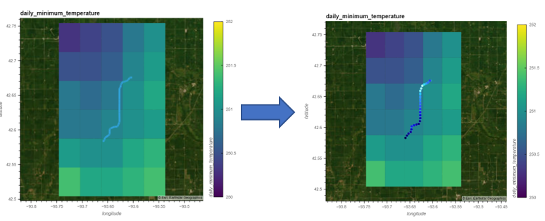
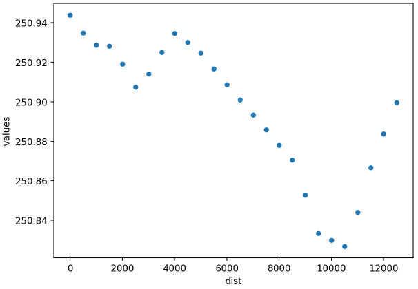
Below is a simple plot showing the values of the inerpolated points plotted against the distance of the points.
# Plot values of the interpolated points
pts.plot(kind='scatter', x = 'dist', y='values')
Here the stats dataframe is filtered to show the line statistics for our selected time, line and grid.

# Get stats for line by select for time, geometry, and grid variable
stats1[(stats1[stat_time_column]==time) & (stats1[ID_column]==ID) & (stats1[stat_varname_column]==varname)]| date | permanent_ | varname | mean | median | std | min | max | |
|---|---|---|---|---|---|---|---|---|
| 5 | 1979-01-06 | 155842105 | daily_minimum_temperature | 250.895452 | 250.904224 | 0.034852 | 250.826833 | 250.943885 |
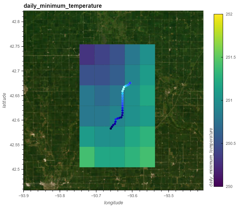
And here is an interactivate map displaying the gridded data, interpolated points and line geometry.
# Display data
from holoviews.element.tiles import EsriImagery

line = gdf[gdf[ID_column]==ID].to_crs(4326).hvplot(
    geo=True, frame_width=600, frame_height=500, alpha=1,  clim=(30, 90),
    xlabel="longitude", ylabel="latitude",  line_width=5,
)

sample_points = pts.to_crs(4326).hvplot(
    c='values', geo=True, frame_width=600, frame_height=500, alpha=1,
    xlabel="longitude", ylabel="latitude", clabel=varname,
    title="Interpolated Points", aspect='equal'
)
gridded_data = da.isel(day=5).hvplot.quadmesh(
    'lon', 'lat', varname, cmap='viridis', alpha=1, grid=True, geo=True, frame_width=500,
    clim=(250, 252), xlabel="longitude", ylabel="latitude", clabel=varname,
    title=varname, aspect='equal'
)

(EsriImagery() * gridded_data * line * sample_points)

