import warnings
warnings.filterwarnings("ignore")
import geopandas as gpd
import pandas as pd
import hvplot.pandas
import hvplot.xarray

import xarray as xr
import pynhd
from pynhd import NLDI, NHDPlusHR, WaterData
from gdptools import UserTiffData
from gdptools import InterpGen
import geoviews as gv

gv.extension('bokeh', 'matplotlib')
# gv.extension()
# gv.output(dpi=120, fig='png')
# gv.output(backend='bokeh')Use Cases
3dep-grid-to-line
Keywords: Interpolation; grid-to-line; 3DEP, Topography; NHD; Stream-segments
Domain: Topography; Stream Characteristics
Language: Python
Description:
In this example, a set of NHD stream-segments accessed using the HyRiver package. A USGS 3DEP Elevation dataset is pulled in using the ClimateR-Catalog. Finally, gdptools is used to interpolate the 3DEP elevation to the NHD stream-segments.
3DEP Elevation Grid-to-line intersection
Introduction
In this example, a set of NHD stream-segments accessed using the HyRiver package. A USGS 3DEP Elevation dataset is pulled in using the ClimateR-Catalog. Finally, gdptools is used to interpolate the 3DEP elevation to the NHD stream-segments.
Geo Data Processing Tools (gdptools)
gdptools is a python package for calculating area-weighted statistics of grid-to-polygon. grid-to-line, and polygon-to-polygon interpolations. gdptools utilizes metadata from the OPeNDAP catalog to aid generalizing gdptools processing capabilities. There are also methods for calculating area-weighted statistics for any gridded dataset that can be opened by xarray, however some of the metadata encapsulated in the json entries will have to be added by the user. Examples can be found in Non-Catalog Examples.
Open Source Python Tools
- xarray: Package to work with labelled multi-dimensional arrays.
- geopandas: Package to work with geospatial data.
Data
- 3DEP: The USGS 3D Elevation Program (3DEP) Datasets are the primary elevation data product produced and distributed by the USGS.
- NHDPlus_V2: National Hydrography Dataset Plus Version 2, a selection of flowline geometries from HUC 0708
Maintenance Schedule
- The intent of this notebook is simply a demonstration of an application or workflow. As we progress in the build-out of NGHF project tools, this notebook may be updated or replaced. There is no other planned maintenance at this time.
Description
This workflow demonstrates the grid to line interpoltion functionality from the gdptools package. The purpose of this tool is to attribute gridded data to line geometries. This is done by interpolating points along each line geometry and extracting the underlaying gridded data values at those points. From this point values, statistics are calculated and attributed to the original input lines.
The inputs to the line interpolation tool are a Geopandas geodataframe containing the line geometries, and a Pandas dataframe containing information about the gridMET gridded data. The line interpolation tool can process multi-dimensional xarray data, outputing the statistics organized by each time segment. Also, multiple gridded datasets can be processed, so for a gridMET example, three different climate variables can be accessed and processed.
The outputs are a dataframe containing the statistics for each line geometries calculated for each gridded dataset at each time segment, as well as a geodataframe containing the interpolated point geometries which have the linearly interpolated values from the gridded dataset. Depending on the user’s inputs, the sample points can be interpolated from the line geometry at regular intervals, or the line vertices can be used instead.
Create conda environment
- gdptools-examples can be downloaded from the project repo
Imports
Create target lines
nldi = NLDI()
station_id = "06730200"

basin = nldi.get_basins(station_id)

flw_main = nldi.navigate_byid(
    fsource="nwissite",
    fid=f"USGS-{station_id}",
    navigation="upstreamMain",
    source="flowlines",
    distance=1000,
)

nhdp_mr = WaterData("nhdflowline_network")
comids = [int(c) for c in flw_main.nhdplus_comid.to_list()]
nhd_mr_fl = nhdp_mr.byid("comid", comids)
nhd_mr_fl.columns.to_list()
flw = pynhd.prepare_nhdplus(nhd_mr_fl, 0, 0, purge_non_dendritic=True)
flw2 = flw.rename(columns={"comid": "ID", "tocomid": "toID"})
strm_segs = pynhd.topoogical_sort(flw2)

# copy the sorted comids into a list and remove the last element
# List will be used to sort ouput into topological order later
sort_ids = strm_segs[0]

# create a new dataframe with the sorted comids
mr_fl = nhd_mr_fl.set_index("comid").loc[sort_ids[:-1]]
mr_fl = mr_fl.reset_index()

mr_fl.head()| comid | geometry | fdate | resolution | gnis_id | gnis_name | lengthkm | reachcode | flowdir | wbareacomi | ... | qc_12 | vc_12 | qe_12 | ve_12 | lakefract | surfarea | rareahload | rpuid | vpuid | enabled | |
|---|---|---|---|---|---|---|---|---|---|---|---|---|---|---|---|---|---|---|---|---|---|
| 0 | 2889852 | MULTILINESTRING Z ((-105.63211 40.05203 0.0000... | 2000-12-22T05:00:00Z | Medium | 178467 | North Boulder Creek | 0.373 | 10190005000122 | With Digitized | 2888392 | ... | 0.376 | -9998.00000 | 0.376 | -9998.00000 | 1.0 | 50667.042715 | 10.004544 | 10c | 10L | 1 |
| 1 | 2889186 | MULTILINESTRING Z ((-105.62824 40.05363 0.0000... | 1999-05-28T04:00:00Z | Medium | 178467 | North Boulder Creek | 0.552 | 10190005000121 | With Digitized | 0 | ... | 0.498 | 0.57306 | 0.498 | 0.57306 | NaN | NaN | NaN | 10c | 10L | 1 |
| 2 | 2889770 | MULTILINESTRING Z ((-105.62207 40.05389 0.0000... | 1999-05-28T04:00:00Z | Medium | 178467 | North Boulder Creek | 0.478 | 10190005000120 | With Digitized | 2888388 | ... | 0.592 | -9998.00000 | 0.592 | -9998.00000 | 1.0 | 52090.136727 | 6.691098 | 10c | 10L | 1 |
| 3 | 2889188 | MULTILINESTRING Z ((-105.61719 40.05556 0.0000... | 1999-05-28T04:00:00Z | Medium | 178467 | North Boulder Creek | 0.396 | 10190005000119 | With Digitized | 0 | ... | 0.659 | 0.62836 | 0.659 | 0.62836 | NaN | NaN | NaN | 10c | 10L | 1 |
| 4 | 2889772 | MULTILINESTRING Z ((-105.61573 40.05258 0.0000... | 1999-05-28T04:00:00Z | Medium | 178467 | North Boulder Creek | 0.257 | 10190005000118 | With Digitized | 2888396 | ... | 0.785 | -9998.00000 | 0.785 | -9998.00000 | 1.0 | 48345.911611 | 4.708286 | 10c | 10L | 1 |
5 rows × 138 columns
Plot the target lines
from bokeh.models import PrintfTickFormatter
formatter = PrintfTickFormatter(format="%i")
gv.tile_sources.EsriTerrain * gv.Path(mr_fl.to_crs(4326), vdims="comid").opts(color='comid',cmap='category20', width=600, height=300, aspect="equal", line_width=5, show_legend=True, colorbar=True, colorbar_opts={'formatter': formatter}, clabel="segment ID", title="NHDPlus MR Flowlines upstream of USGS Gage 06730200")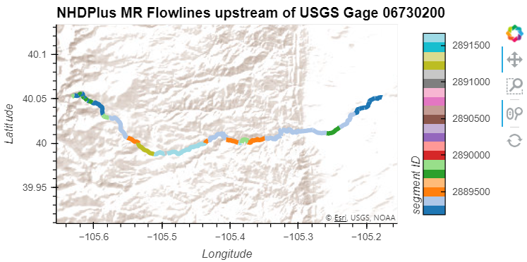
Define source data
import pprint
climater_cat = "https://mikejohnson51.github.io/climateR-catalogs/catalog.parquet"
cat = pd.read_parquet(climater_cat)

_id = "USGS 3DEP"
_asset = "10m CONUS DEM"
_vars = ["elevation"]
# create list of catalog parameters for each variable
cat_params = [
    cat.query("id == @_id & asset == @_asset & variable == @_vars").to_dict(orient="records")[0]
    for _var in _vars
]
# create dictionary of variable names and catalog parameters
cat_dict = dict(zip(_vars, cat_params))
pprint.pprint(cat_dict)
{'elevation': {'T_name': None,
'URL': '/vsicurl/https://prd-tnm.s3.amazonaws.com/StagedProducts/Elevation/13/TIFF/USGS_Seamless_DEM_13.vrt',
'X1': -180.0005555560936,
'X_name': None,
'Xn': 180.00000026239937,
'Y1': -180.0005555560936,
'Y_name': None,
'Yn': 72.0005555562949,
'asset': '10m CONUS DEM',
'crs': '+proj=longlat +datum=NAD83 +no_defs',
'description': '10m CONUS DEM',
'duration': None,
'ensemble': None,
'id': 'USGS 3DEP',
'interval': None,
'model': None,
'nT': nan,
'ncols': 3888006.0,
'nrows': 939612.0,
'resX': 9.259259266022042e-05,
'resY': 9.25925926599094e-05,
'scenario': None,
'tiled': '',
'toptobottom': None,
'type': 'vrt',
'units': 'meters',
'variable': 'elevation',
'varname': 'elevation'}}Load source data
import rioxarray as rxr
ds_3dep = rxr.open_rasterio(cat_dict["elevation"]["URL"])
ds_3dep
<xarray.DataArray (band: 1, y: 939612, x: 3888006)> Size: 15TB
[3653217093672 values with dtype=float32]
Coordinates:
* band (band) int64 8B 1
* x (x) float64 31MB -180.0 -180.0 -180.0 ... 180.0 180.0 180.0
* y (y) float64 8MB 72.0 72.0 72.0 72.0 ... -15.0 -15.0 -15.0 -15.0
spatial_ref int64 8B 0
Attributes:
_FillValue: -999999.0
scale_factor: 1.0
add_offset: 0.0Define UserTiffData object
varname = "elevation"
tx_name = "x"
ty_name = "y"
band = 1
bandname = "band"
crs = 4269
f_crs = 4326
id_feature = "comid"
user_data = UserTiffData(
    var=varname,
    ds=ds_3dep,
    proj_ds=crs,
    x_coord=tx_name,
    y_coord=ty_name,
    band=band,
    bname=bandname,
    f_feature=mr_fl,
    id_feature=id_feature,
    proj_feature=crs
)
Define InterpGen object and generate interpolation
interpObject1 = InterpGen(user_data, pt_spacing=100, stat='all', interp_method="linear")
# stats1, pts1 = interpObject1.calc_interp()
stats1, pts1 = interpObject1.calc_interp()Plot the sub-setted 3DEP 10m DEM
ds_ss = user_data.get_source_subset(key="").to_dataset(name="elevation")
ds_ss.elevation.hvplot.quadmesh(x="x", y="y", geo=True, project=True, rasterize=True,  cmap="viridis", width=600, height=300, aspect="equal", clabel="3DEP 10m DEM", xlabel="Longitude", ylabel="Latitude", title="3DEP 10m DEM")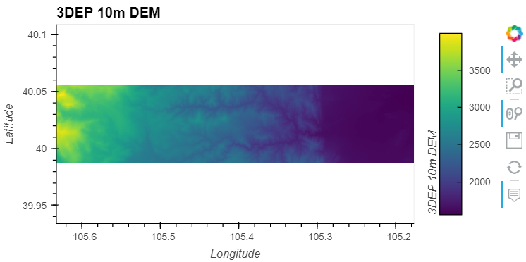
Show the interpolated points
pts1.head(10)| band | spatial_ref | values | dist | comid | geometry | varname | |
|---|---|---|---|---|---|---|---|
| pt | |||||||
| 0 | 1 | 0 | 3620.148240 | 0.0 | 2889186 | POINT (-105.62824 40.05363) | elevation |
| 1 | 1 | 0 | 3620.536633 | 100.0 | 2889186 | POINT (-105.62721 40.05347) | elevation |
| 2 | 1 | 0 | 3605.426694 | 200.0 | 2889186 | POINT (-105.62617 40.05330) | elevation |
| 3 | 1 | 0 | 3589.268663 | 300.0 | 2889186 | POINT (-105.62513 40.05317) | elevation |
| 4 | 1 | 0 | 3578.737594 | 400.0 | 2889186 | POINT (-105.62408 40.05319) | elevation |
| 5 | 1 | 0 | 3571.558704 | 500.0 | 2889186 | POINT (-105.62307 40.05350) | elevation |
| 6 | 1 | 0 | 3561.002180 | 600.0 | 2889186 | POINT (-105.62208 40.05386) | elevation |
| 0 | 1 | 0 | 3562.425944 | 0.0 | 2889188 | POINT (-105.61719 40.05555) | elevation |
| 1 | 1 | 0 | 3560.132325 | 100.0 | 2889188 | POINT (-105.61623 40.05523) | elevation |
| 2 | 1 | 0 | 3524.454683 | 200.0 | 2889188 | POINT (-105.61593 40.05429) | elevation |
Show The statistics
stats1.head(10)| comid | varname | mean | median | std | min | max | |
|---|---|---|---|---|---|---|---|
| 0 | 2889186 | elevation | 3592.382673 | 3589.268663 | 21.869669 | 3561.002180 | 3620.536633 |
| 0 | 2889188 | elevation | 3530.434588 | 3542.293504 | 35.512939 | 3474.725399 | 3562.425944 |
| 0 | 2889198 | elevation | 3448.163413 | 3448.163413 | 5.088796 | 3443.074617 | 3453.252209 |
| 0 | 2889214 | elevation | 1558.948775 | 1558.909872 | 1.177188 | 1556.995957 | 1560.632596 |
| 0 | 2889222 | elevation | 3383.079157 | 3384.111947 | 20.186174 | 3357.856033 | 3407.269491 |
| 0 | 2889228 | elevation | 1562.467656 | 1562.329510 | 1.200723 | 1560.514657 | 1564.282919 |
| 0 | 2889258 | elevation | 1566.994847 | 1567.276408 | 1.405514 | 1564.551618 | 1569.605378 |
| 0 | 2889260 | elevation | 1570.061488 | 1569.926930 | 1.177132 | 1568.664825 | 1572.449691 |
| 0 | 2889264 | elevation | 1572.780286 | 1572.780286 | 0.221680 | 1572.558607 | 1573.001966 |
| 0 | 2889276 | elevation | 1574.920887 | 1574.883109 | 1.282772 | 1572.988032 | 1576.906272 |
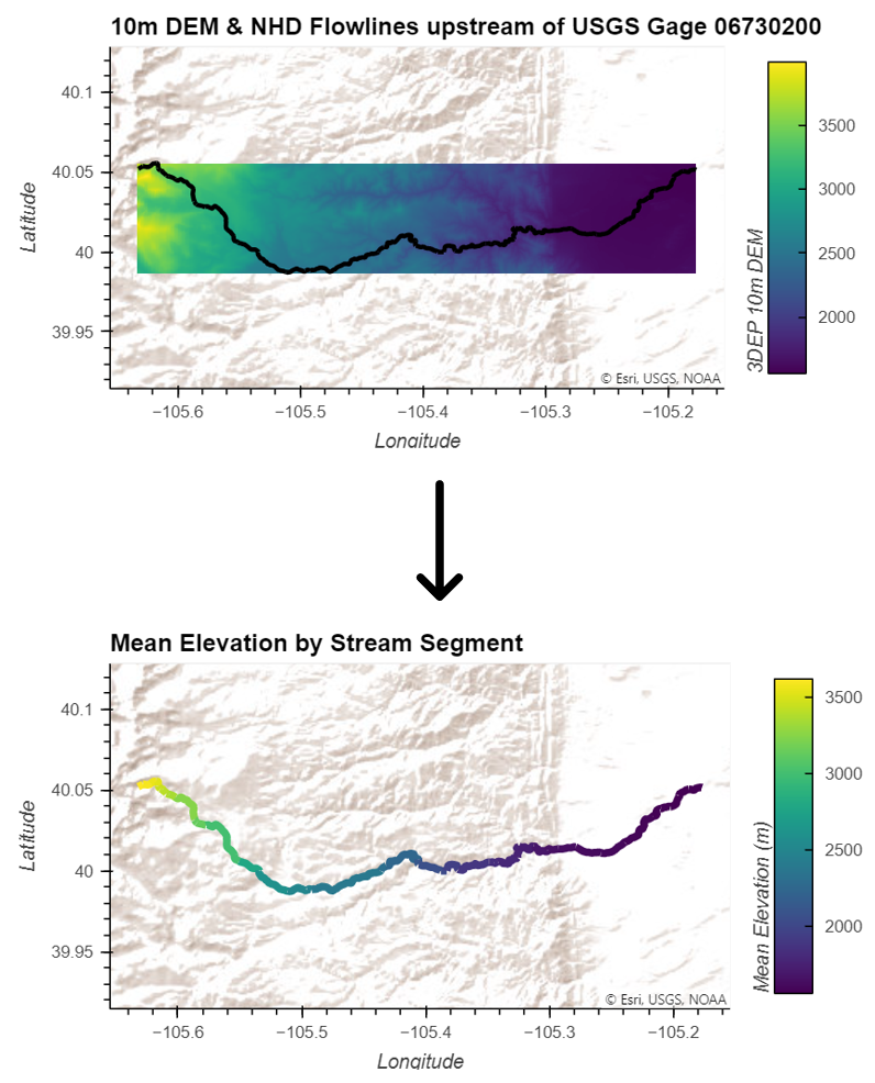
Plot the mean elevation by comid
# sort stats by topological stream order
stats = stats1.set_index("comid").loc[sort_ids[:-1]]
mr_fl["tmean"] = stats["mean"].values
pmin = mr_fl["tmean"].min()
pmax = mr_fl["tmean"].max()
pmin, pmax
import geoviews as gv

gv.extension("bokeh")
gv.tile_sources.EsriTerrain * gv.Path(mr_fl.to_crs(4326), vdims=["tmean"]).opts(width=600, height=300, aspect="equal",color="tmean", cmap="viridis", line_width=5, colorbar=True, clim=(pmin, pmax), clabel="Mean Elevation (m)", title="Mean Elevation by Stream Segment")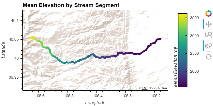
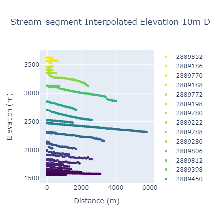
Plot the interpolated data as a scatter plot by comid
import plotly.graph_objects as go
fig = go.Figure()
pts = pts1.groupby("comid")
for index in range(len(pts)):
    group = pts.get_group(sort_ids[index])
    fig.add_trace(go.Scatter(x=group["dist"], y=group["values"], mode='markers', marker=dict(size=5, color=group["values"], colorscale='Viridis', cmin=pmin, cmax=pmax), name=str(sort_ids[index])))
fig.update_layout(title="Stream-segment Interpolated Elevation 10m DEM", xaxis_title="Distance (m)", yaxis_title="Elevation (m)")
fig.show()