 |
|
|
||||
| Scientific Investigations Report 2005–5030 |
In cooperation with the Menominee Indian Tribe of Wisconsin

Figure 1. Location of valley transects, stream gages, and precipitat...
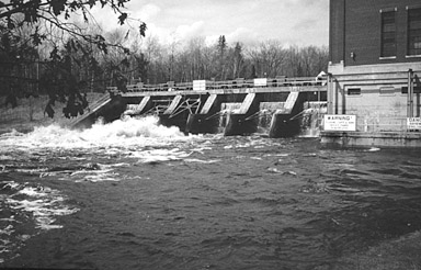
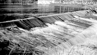
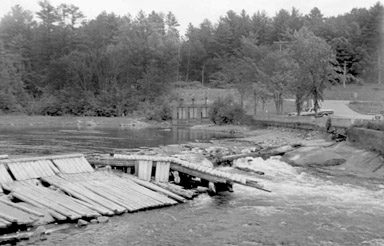
Figure 2. Photos of A, Balsam Row Dam in 1998, looking upstream at d...
Figure 3. Longitudinal profile of the Wolf River through the Menomin...
Figure 4. Boxplots of A, mean daily streamflow, and B, annual peak f...
Figure 5. Annual peak streamflow from the Wolf River near Shawano (t...
Figure 6. Annual peak flow and trend lines for the Wolf River near S...
Figure 7. Annual precipitation and trend lines for Green Bay, Wis., ...
Figure 8. Trace of the Wolf River, Wis., showing channel position in...
Figure 9. Detailed longitudinal profile of the Wolf River from the B...
Figure 10. Valley transect through the impounded reach of the Wolf R...
Figure 11. Valley transect through the impounded reach of the Wolf R...
Figure 12. Valley transect through the impounded reach of the Wolf R...
Figure 13. Data for 137Cs, unsupported 210Pb, and ...
Figure 14. Profiles for A, particle-size distribution, B, bulk densi...
Figure 15. Valley transect through the impounded reach of the Wolf R...
Figure 16. Valley transect through the sandy reach of the Wolf River...
Figure 17. Partial valley transect through the sandy reach of the Wo...
Figure 18. Partial valley transect through the sandy reach of the Wo...
Figure 19. Valley transect through the sandy reach of the Wolf River...
Figure 20. Valley transect through the rocky reach of the Wolf River...
Figure 21. Ice damage on trees in flood plain near transect T9, Apri...
Figure 22. Selected profiles of trace elements for core T2-1 from th...
Table 1. U.S. Geological Survey stream gages used in the analyses of...
Table 2. Description of valley transects and cores collected along t...
Table 3. Summary of core locations, water depths, penetration depths...
Table 4. Selected trend-test results for streamflow and precipitation...
Table 5. Water-weight percent, organic-matter content, and dry-bulk ...
Table 6. Minor- and trace-element concentrations and particle size f...
| Multiply | By | To obtain |
|---|---|---|
| Length | ||
| inch (in.) | 2.54 | centimeter (mm) |
| foot (ft) | 0.3048 | meter (m) |
| mile (mi) | 1.609 | kilometer (km) |
| Area | ||
| acre | 0.4047 | hectare (ha) |
| square foot (ft2) | 0.09290 | square meter (m2) |
| square mile (mi2) | 2.590 | square kilometer (km2) |
| Sedimentation and flow rates | ||
| foot per year (ft/y) | 30.48 | centimeter per year (cm/y) |
| cubic foot per second (ft3/s) | 0.02832 | cubic meter per second (m3/s) |
| Mass | ||
| ounce, avoidupois (oz) pound, avoidupois (lb) | 28.35 0.4536 | gram (g) kilogram (kg) |
| Density | ||
| pound per cubic foot (lb/ft3) | 16.02 | kilogram per cubic meter (kg/m3) |
| Radioactivity | ||
| picocurie per liter (pCi/L) | 0.037 | becquerel per liter (Bq/L) |
| Hydraulic gradient | ||
| foot per mile (ft/mi) | 0.1894 | meter per kilometer (m/km) |
Temperature in degrees Fahrenheit (°F) can be converted to degrees Celsius (°C) as follows:
°C = (°F-32)/1.8
Vertical coordinate information is referenced to the National Geodetic Vertical Datum of 1929 (NGVD 29).
Altitude, as used in this report, refers to distance above the vertical datum.
Concentrations of minor and trace elements in sediment are given either in percent or micrograms per gram (mg/g).
Densities are given either as pounds per cubic foot (lb/ft3) or grams per cubic centimeter (g/cm3).
Historical trends in streamflow, sedimentation, and sediment chemistry of the Wolf River were examined for a 6-mile reach that flows through the southern part of the Menominee Indian Reservation and the northern part of Shawano County, Wis. Trends were examined in the context of effects from dams, climate, and land-cover change. Annual flood peaks and mean monthly flow for the Wolf River were examined for 1907–96 and compared to mean annual and mean monthly precipitation. Analysis of trends in sedimentation (from before about 1850 through 1999) involved collection of cores and elevation data along nine valley transects spanning the Wolf River channel, flood plain, and backwater and impounded areas; radioisotope analyses of impounded sediment cores; and analysis of General Land Office Survey Notes (1853–91). Trends in sediment chemistry were examined by analyzing samples from an impoundment core for minor and trace elements. Annual flood peaks for the Wolf River decreased during 1907–49 but increased during 1950–96, most likely reflecting general changes in upper-atmospheric circulation patterns from more zonal before 1950 to more meridional after 1950. The decrease in flood peaks during 1907–49 may also, in part, be due to forest regrowth. Mean monthly streamflow during 1912–96 increased for the months of February and March but decreased for June and July, suggesting that spring snowmelt occurs earlier in the season than it did in the past. Decreases in early summer flows may be a reflection earlier spring snowmelt and large rainstorms in early spring rather than early summer. These trends also may reflect upper-atmospheric circulation patterns. The Balsam Row Dam impoundment contains up to 10 feet of organic-rich silty clay and has lost much of its storage capacity. Fine sediment has accumulated for 1.8 miles upstream from the Balsam Row Dam. Historical average linear and mass sedimentation rates in the Balsam Row impoundment were 0.09 feet per year and 1.15 pounds per square foot per year for 1927–62 and 0.10 feet per year and 1.04 pounds per square foot per year for 1963–99. Sedimentation in the impoundment was episodic and was associated with large floods, especially the flood-related failure of the Keshena Falls Dam in 1972 and a large flood in 1973. Sand deposition is common in the Wolf River upstream from the impounded reach for 2.5 miles and is caused by the base-level increase associated with the Balsam Row Dam. Some sand deposition also may have been associated with logging and log drives in the late 1800s and the failure of the Keshena Falls Dam. In the upstream 1.5-mile part of the studied reach, the substrate is mainly rocky; however, about 2,000 feet downstream from Keshena Falls, the channel has narrowed and incised since the 1890s, likely related to human alterations associated with logging, log drives, and (or) changes in hydraulics and sediment characteristics associated with completion of the Keshena Falls Dam and head race in 1908. Minor- and trace-element concentrations in sediment from Balsam Row impoundment and other depositional areas along the Wolf River generally reflect background conditions as affected by watershed geology and historical inputs from regional and local atmospheric deposition.
The Wolf River is a recreationally and economically important natural resource for the Menominee Indian Tribe of Wisconsin. A study was begun in 1998 by the U.S. Geological Survey (USGS), in cooperation with the Menominee Indian Tribe, to examine historical trends in streamflow, sedimentation, and sediment chemistry of a 6-mi reach of the Wolf River as it flows through the southern part of the Menominee Indian Reservation and northern part of Shawano County, Wis. (fig. 1). For 24 mi upstream from Keshena Falls, the Wolf River was designated a Federal Wild and Scenic River in 1968. The State of Wisconsin also designated the river an Outstanding Resource Water in 1988.
Two dams, the Balsam Row Dam and the failed dam at Keshena Falls, form the lower and upper boundary of the studied reach and have affected channel characteristics in the reach (figs. 1–2). The Keshena Falls Dam failed in 1972 (fig. 2C). Anecdotal evidence from local residents suggests that sedimentation rates in the impoundment above the Balsam Row Dam and sand deposition in the free-flowing reach upstream of the impoundment have accelerated in the last three decades, possibly coincident with the failure of the Keshena Falls Dam. Flooding-related ice jams in winter also have been a problem in the town of Keshena after the failure of the Keshena Falls Dam (U.S. Army Corps of Engineers, 1995).
The goals of this study were to (1) describe historical trends (for the last 100 years or more) in streamflow, sedimentation, and sediment-chemistry characteristics for the Wolf River and (2) identify major factors affecting flooding, sedimentation, and sediment-chemistry characteristics. Data collected as part of this study were useful for determining long-term and upstream/downstream effects from dams on channel characteristics of the Wolf River. Data are useful for establishing baseline conditions in case of future changes in hydrology, sedimentation, or sediment chemistry. Results from the study also provide information for protection or management of available resources, including water quantity, water quality, and aquatic habitat.
This report presents the results from the study of historical trends in streamflow, sedimentation, and sediment chemistry for a 6-mi reach of the Wolf River between the Balsam Row Dam in Shawano County and Keshena Falls in the Menominee Reservation (fig. 1). Trends are described for annual flood peaks and mean monthly flow for the Wolf River based on about 90 years of combined data (1907–96) from two USGS stream gages—Keshena Falls and the Balsam Row Dam (near Shawano). Annual flood peaks during 1968–96 from the stream gage near Shawano were compared to flood peaks at an upstream gage on the Wolf River near Langlade, Wis. Precipitation data from three nearby precipitation stations for 1907–96 are compared to the streamflow trends. Sedimentation patterns in channel, backwater, flood-plain, and impounded areas, historical sedimentation rates, and channel changes are described for a period from about 1850 (pre-European settlement) to 1999. Lastly, minor- and trace-element concentrations in impounded, backwater, and flood-plain sediment are described in terms of historical trends (about 1850–1999) and spatial distribution. This report attempts to evaluate the effects of climate change, logging, forest regrowth, and dams on trends in streamflow, sedimentation, and sediment chemistry over the historical period of interest.
The Wolf River upstream of the Balsam Row Dam has a drainage area of 816 mi2 and has a temperate, continental climate characterized by large seasonal changes in temperature but little variation in monthly precipitation. The Wolf River Basin is typified by an average annual temperature of 43°F, about 30 in. of annual precipitation, 48 in. of annual snowfall, and 18 in. of annual evapotranspiration (Wendland and others, 1985; Olcott, 1968).
The reach of the Wolf River included in this study (fig. 1) generally flows south through coarse-grained glacial deposits and outwash (Clayton and others, 1991; Milfred and others, 1967). These deposits are underlain by Precambrian granite and syenite rocks associated with the Wolf River Complex (Mudrey and others, 1982). Rocks associated with the Wolf River Complex crop out at Keshena Falls but are buried by glacial, outwash, and fluvial deposits to the south and through most of the study reach.
Flood-plain soils near the Wolf River are characterized as loamy Fluvaquents or Fluvents and are underlain by coarse- and fine-grained deposits associated with outwash plains or glacial lakes (Gundlach and others, 1982). The flood-plain soils generally contain about an 8-in. thick organic surface layer, although some have as much as 15 in. of organic-rich loam at the surface. Upland soils near the studied reach are well-drained sandy or loamy Spodosols or Alfisols (Gundlach and others, 1982).
The slope of the Wolf River is highly variable through the Menominee Indian Reservation but flattens out considerably below Keshena Falls (fig. 3). Based on measurements of stream length and contour intervals from USGS 7.5-minute topographic maps, the average slope is 11.6 ft/mi from the headwaters to Big Smoky Falls, and the average slope from Big Smoky Falls to Keshena Falls is 4.9 ft/mi. In contrast, the average slope is 2.0 ft/mi downstream from Keshena Falls to the Balsam Row Dam.
Figure 3. Longitudinal profile of the Wolf River through the Menominee Indian Reservation, Wis.
Land cover in the Wolf River Basin upstream from the Balsam Row Dam is mainly forest (72 percent of the basin) and wetland (15 percent) as inferred from 1992–93 satellite imagery (Reese and others, 2002). Cropland accounts for only 4 percent of the drainage area. Of the forested land, 78 percent is deciduous (mainly aspen and maple), 16 percent is mixed deciduous and conifer, and 6 percent is conifer. Along the study reach, vegetation in the upland generally is categorized as pine plantation (Milfred and others, 1967). The Menominee Indian Tribe has used selective logging and sustainable forestry techniques on their lands since the reservation was established in 1854 (Menominee Tribal Enterprises, 1997). The reservation covers the lower third of the Wolf River Basin (fig. 1). Most of the upper part of the basin was logged before 1900 (Connor, 1978). The Wolf River and its tributaries were used for transportation of saw logs from the upper basin to Shawano and further downstream during the late 1800s (Oehmcke and Truax, 1964; Connor, 1978). Logging in the area peaked in 1873.
In the late 1800s the upper Wolf River had various small dams related to logging and log drives (Smith, 1908; U.S. Department of Agriculture and the University of Wisconsin, 1961). Both the Keshena Falls Dam and the Balsam Row Dam were used for hydroelectric power generation. Neither dam has flood-control function. The presence of some sort of dam structure at Keshena Falls dates back to the 1870s and was related to logging, but the most recent dam was constructed in 1906–08 and failed in 1972 (Wisconsin Department of Natural Resources, Dam File No. 72.1, Madison, Wis.). The Keshena Falls Dam had about 16 ft of head. The dam consisted of two parts—a wooden apron that extended across the main channel of the Wolf River and four gates across a diversion canal (head race) for the powerplant (fig. 2B). The failure of the Keshena Falls Dam in 1972 happened after about 9 years of disrepair along the left side of the wooden spillway apron (Wisconsin Department of Natural Resources, Dam File No. 72.1, Madison, Wis.) (fig. 2C).
The Balsam Row Dam (fig. 2A) was constructed in 1927 and there is no indication of any earlier version of a dam at Balsam Row before then (Smith, 1908). The Balsam Row Dam has six gates and about 14 ft of head. The powerhouse is on the east side of the dam embankment next to the gates.
A general description of the surface-water and ground-water quality for the Menominee Indian Reservation was previously published in Krohelski and others (1994). Garn and others (2001) provide additional data on the quality of water, sediment, and selected benthic organisms from the Wolf River during 1986–98.
This study involved collecting and compiling historical records as well as collecting new field data. General Land Office Survey notes provided information on channel characteristics before and during European settlement, logging, and log drives in the mid to late 1800s.
Streamflow trend analyses involved statistical examination of trends in annual peak and average monthly flow data from a former USGS stream gage at the Balsam Row Dam near Shawano, Wis. (USGS station number 04077400), with 93 years of data (1907–09, 1910–2001). The stream gage was moved from Keshena Falls to the Balsam Row Dam in 1985 (table 1). Mean daily flow data were examined before and after the site location changed to confirm that streamflow characteristics were the same at both locations. Annual peak data from the Shawano site also were compared to data from the Wolf River near Langlade, Wis. (USGS station number 04074950). The drainage area of the Wolf River at Langlade is about half that of the Wolf River near Shawano (table 1). Trend analysis was also done on annual and monthly precipitation from three nearby National Weather Service climate stations (Rhinelander, Shawano, and Green Bay, Wis.) over the same period to identify climatic effects on streamflow characteristics.
[mi2, square miles]
| Station name | USGS station identification number (fig. 1) | Period of record | Drainage area (mi2) |
|---|---|---|---|
| Wolf River at Balsam Row Dam near Shawano, Wis. | 04077400 | 1985–2001 | 816 |
| Wolf River at Keshena/Keshena Falls, Wis. | 04077000 | 1907–09,1910–85 | 788 |
| Wolf River at Langlade, Wis. | 04074950 | 1968–present | 463 |
Analysis of historical changes in sedimentation and sediment quality involved collection of cores and elevation data along nine valley transects spanning the Wolf River channel, flood plain, and impounded area above the Balsam Row Dam from February through June 1999 (table 2). Locations of transects are shown in figure 1. The number of cores collected along each transect varied because of differences in the number of depositional environments found along each transect. For example, transect T4.2 was along a stretch of the Wolf River with no flood plain and a uniform sand channel bottom. In contrast, transect T7 intersected a longitudinal bar, a backwater channel, and flood-plain deposits and required more cores for an adequate description of the range of fluvial environments traversed. Sediment samples were selected from cores of the various environments and analyzed for sediment chemistry, radiometric age dating, and particle-size distribution. In November 2001, a second core was collected near core T2-1 to obtain additional information on water, organic-matter content, and dry-bulk density.
[Distances are curvilinear channel distances; ft, feet]
| Transect (fig. 1) | Description | Distance upstream of Balsam Row Dam (ft) | Distance along longitudinal profile (ft) (fig. 9) | Number of cores collected | Number of duplicate cores collected | Cores sampled for laboratory analyses |
|---|---|---|---|---|---|---|
| T1b | Impoundment | 450 | 1,850 | 3 | 0 | None |
| T1c | Impoundment | 860 | 2,260 | 3 | 0 | None |
| T2 | Impoundment | 1,390 | 2,790 | 4 | 1 | T2-1 |
| T3 | Cedar wetland, rice beds, water impounded but some current | 5,650 | 7,050 | 4 | 0 | None |
| T4 | County line, large backwater area on left side | 9,690 | 11,090 | 10 | 4 | T4-7, T4-9 |
| T4.2 | Sand deposition in channel | 13,530 | 14,930 | 4 | 0 | None |
| T4.5 | Sand deposition in channel | 13,980 | 15,380 | 1 | 0 | None |
| T51 | Sand deposition in channel | 15,200 | 16,600 | 3 | 0 | None |
| T61 | Sand deposition in channel | 17,500 | 18,900 | 2 | 0 | None |
| T7 | Large depositional bar on right side of channel | 20,440 | 21,840 | 17 | 4 | T7-2, T7-3, T7-12 |
| T9 | Wide flood plain | 28,570 | 29,970 | 12 | 7 | T9-2 |
1 No valley transect surveys were done for T5 and T6.
General Land Office (GLO) Surveys were done in the mid 1800s across Wisconsin to map and establish townships, ranges, and sections. In northern Wisconsin, these surveys usually were done before European settlement and were useful for characterizing stream conditions before widespread logging and burning coincident with European settlement in the late 1800s. Copies of original GLO survey notes were obtained from the State of Wisconsin, Board of Commissioners of Public Lands for two townships: Township 27 North, Range 15 East, and Township 28 North, Range 15 East. The surveys were done from 1845 through 1891, with notes for the south boundary of Township 28 from 1845, Township 27 from 1853, and Township 28 from 1891.
Field notes from the GLO Surveys contain information on vegetation, soils, and the lay of the land, as well as the location, width, depth, substrate, swiftness of flow, and direction of streams at section-line crossings. These notes were used to determine the location of the Wolf River channel before the impoundment of water behind the Balsam Row Dam. Meander data for the Wolf River also were reported; these data described the location of both streambanks longitudinally.
Data from two USGS stream gages on the Wolf River were examined for trends in annual flood peaks and mean monthly flow: the Wolf River near Shawano (the Balsam Row Dam) and the Wolf River near Langlade (fig. 1, table 1). The gage near Shawano was moved from Keshena Falls to the Balsam Row Dam in 1985 and was operated at the Balsam Row Dam until 2001. Streamflow data for the two gages were combined and recorded under site 04077400 in USGS databases because of similar drainage areas (table 1). Annual flood peaks for the combined record are available for 1907–09 and 1910–96. Mean monthly data are available for 1912–96. Mean daily flow and annual peaks from 1975–85 and 1985–95 were examined for differences by use of two-sample t-tests with log-transformed data and the nonparametric Wilcoxon rank sum test (Iman and Conover, 1983). Gebert and Krug (1996) also combined data from the Balsam Row Dam and Keshena Falls gages and examined trends in annual flood peaks and low flow for the period of record 1931–91.
Tests for normal distributions of the data were performed and log transformations were used to normalize the data. The log-transformed data were analyzed for trends by use of the least squares method for linear regression (Iman and Conover, 1983). Slopes in the trend lines were considered statistically significant if p-values were less than 0.10. Trend analyses were done on annual peak flow and mean monthly data for 1907–96 and also divided into pre- and post-1950 periods because hemispheric-scale climate change is thought to have occurred around 1950 (Knox and others, 1975; Kalnicky, 1974). Although highly variable and season-dependent, upper atmospheric circulation patterns generally changed from more zonal (west-east) before 1950 to more meridional (north-south) after 1950. Changes in upper atmospheric circulation in Wisconsin affect the frequency, intensity, and seasonality of precipitation (Knox and others, 1975). Meridional patterns tend to produce more floods on an annual basis than any other circulation pattern. Zonal patterns tend to produce mild weather in the Great Lakes region (Eichenlaub, 1979).
Annual precipitation data from three long-term climate stations (Rhinelander, Shawano, and Green Bay, fig. 1) were obtained from the State Climatologist's Office in Madison, Wisconsin. The stations are operated by the National Weather Service. The Rhinelander station had data beginning in 1908. Precipitation records for Shawano began in 1923 and for Green Bay began in 1912. Trend analyses (least squares method for linear regression) were done on average annual and average monthly precipitation data in the same fashion as was done with the streamflow data.
Data collected from valley transect surveys and sediment coring were used to determine historical sedimentation rates and historical trends in sediment chemistry. A reconnaissance trip was done in October 1998 along the Wolf River from Keshena Falls to the Balsam Row Dam to identify possible transects for sediment coring. Nine transects (fig. 1; table 2) were selected along the study reach and numbered in upstream order, the starting point being at the Balsam Row Dam. Transects were located in reaches with a flood plain and with depositional zones within the channel. Transects were surveyed in May and June 1999 by use of an auto level. A global positioning system was used to verify the location of each transect. Elevation data were tied into U.S. Army Corps of Engineers reference marks from a flood-plain delineation study done in 1995 (U.S. Army Corps of Engineers, 1995). Soft- and hard-bottom elevations for transect T1b, T1c, T2, T3, and T4 were collected by use of a sounding pole in unwadeable areas. Hard-bottom elevations are assumed to be elevations of pre-dam sediment surfaces (streambed, streambank, backwater, or flood plain). No valley-transect surveys were done at T5 and T6; only exploratory cores from channel deposits were collected during the reconnaissance trip.
The thickness, texture, chemistry, and age of sediment in the flood plain, backwater areas, impoundment, and modern channel were examined by sediment coring and sampling with four devices, including a 1-in.-diameter hand-held soil probe, a geoprobe, and two types of piston corers—the Wisconsin Department of Natural Resources (WDNR) corer (3-in. diameter) and the modified Livingston corer (2-in. diameter) (table 3). The hand-held soil probe was useful for quick exploratory coring of flood-plain deposits and field sediment descriptions. The geoprobe is a tapping-type coring device that was mounted on a four-wheel all-terrain vehicle and was used to collect cores from the impounded reach when it was frozen and from accessible flood-plain areas. The WDNR corer is limited to depths less than about 2 m and was used to collect cores from inundated areas. The modified Livingston was used to collect multiple cores at depth from fine-grained deposits (Wright, 1967).
[ft, feet; LB, left bank; WDNR, Wisconsin Department of Natural Resources; te, minor and trace elements; cs, 137Cs and 210Pb radiometric dating; ps, particle size; RP1, Reference point (survey stake) for transect endpoint; LEW, left edge of water; u.s., upstream; wd, radiocarbon; --, not measured]
| Core | Description | Water depth (ft) | Penetration depth (ft) | Samples saved | Sample analyses | Type of core | Site file established |
|---|---|---|---|---|---|---|---|
| Transect T1b | |||||||
| 1 | 138 feet west of LB, impoundment | 4.9 | 4.9 | no | no | WDNR piston | no |
| 2 | 276 feet west of LB, impoundment | 6.6 | 5.1 | no | no | WDNR piston | no |
| 3 | 414 feet west of LB, impoundment | 6.0 | 12.1 | no | no | WDNR piston, Livingston | no |
| Transect T1c | |||||||
| 1 | 150 feet west of LB, impoundment | 4.9 | 13.4 | no | no | WDNR piston, Livingston | no |
| 2 | 300 feet west of LB, impoundment | 6.6 | 8.4 | no | no | WDNR piston, Livingston | no |
| Transect T2 | |||||||
| 1 | 150 feet west of LB, impoundment | 6.2 | 8 | te, cs, ps | te, cs, ps | WDNR piston, geoprobe, Livingston | Feb-99 |
| 2 | 300 feet west of LB, impoundment | 2.3 | 4.2 | yes | no | WDNR piston | no |
| 3 | 450 feet west of LB, impoundment | 5.2 | 4.9 | yes | no | WDNR piston | no |
| 4 | 600 feet west of LB, impoundment | 8.05 | 3.1 | yes | no | WDNR piston | no |
| Transect T4 | |||||||
| 1 | 200 feet right of RP1, hayfield, terrace | 0 | 29 | core | no | Geoprobe | no |
| 2 | 100 feet right of RP1, hayfield, terrace | 0 | 22 | core | no | Geoprobe | no |
| 3 | 10.5 feet right of RP1, hayfield, flood plain | 0 | 29 | core | no | Geoprobe | no |
| 4 | 300 feet right of RP1, hayfield, base of terrace slope | 0 | 8 | core | no | Geoprobe | no |
| 5 | 400 feet right of RP1, hayfield, base of terrace slope | 0 | 8 | core | no | Geoprobe | no |
| 6 | 186 feet right of LEW, center channel | 6.2 | 1.7 | no | no | WDNR piston | no |
| 7 | 40 feet right of LEW, backwater | 1.4 | 3.6 | no | no | WDNR piston | Sep-99 |
| 7a | 40 feet right of LEW, backwater | 1.4 | 3.4 | te, ps, peat | te, ps, wd | WDNR piston | no |
| 7b | 40 feet right of LEW, backwater | 1.4 | 3.4 | ps, peat, wd | ps, wd | WDNR piston | no |
| 7c | 40 feet right of LEW, backwater | 1.6 | 3.5-5.1 | wd | no | Livingston | no |
| 8 | 80 feet right of LEW, backwater | .8 | 3.6 | no | no | WDNR piston | no |
| 9 | 120 feet right of LEW, backwater | .4 | 3.1 | no | no | WDNR piston | Sep-99 |
| 9a | 120 feet right of LEW, backwater | .3 | 3.2 | te, wd | te, wd | WDNR piston | no |
| 9b | 120 feet right of LEW, backwater | .4 | 3.4 | ps, wd | ps | WDNR piston | no |
| 10 | ~80 feet u.s. of T4-7, backwater | 1.85 | 1.8 | no | no | WDNR piston | no |
| Transect T4.2 | |||||||
| 4.2-1 | 111 feet right of LEW, channel | 2.7 | 2.05 | no | no | WDNR piston | no |
| 4.2-2 | 150 feet right of LEW, channel | 2.7 | 1.4 | no | no | WDNR piston | no |
| 4.2-3 | 90 feet right of LEW, channel | 3.8 | 2.8 | no | no | WDNR piston | no |
| 4.2-4 | 60 feet right of LEW, channel | 4.1 | .15 | no | no | WDNR piston | no |
| Transect T4.5 | |||||||
| 4.5-1 | 150 feet right of LEW, channel | 0.5 | 2.35 | no | no | WDNR piston | no |
| 4.5-2 | 170 feet right of LEW, channel | 1.1 | 2.7 | no | no | WDNR piston | no |
| Transect T5 | |||||||
| 1 | paleochannel | 0.0 | 4.0 | no | no | Oakfield soil probe | no |
| 2 | right side, thalweg | -- | .3 | no | no | Oakfield soil probe | no |
| 3 | left side, channel | -- | 1.75 | no | no | Oakfield soil probe | no |
| Transect T6 | |||||||
| 1 | right side, channel margin, backwater | 0.3 | 2.5 | no | no | Oakfield soil probe | no |
| 2 | right side, channel | -- | .5 | no | no | Oakfield soil probe | no |
| Transect T7 | |||||||
| 1 | 460 feet right of RP1, backwater channel | 0.5 | 3.2 | wd | no | WDNR piston | no |
| 2 | 430 feet right of RP1, backwater channel | 0.9 | 2.1 | ps | ps | WDNR piston | Sep-99 |
| 2a | 430 feet right of RP1, backwater channel | 0.9 | 1.1 | te, cs | te, cs | WDNR piston | no |
| 2b | 430 feet right of RP1, backwater channel | 0.9 | 3.1-4.4 | wd | wd | Livingston | no |
| 3 | 418 feet right of RP1, backwater channel | 0.8 | 2.2 | wd | no | WDNR piston | no |
| 3a | 418 feet right of RP1, backwater channel | 0.8 | 2.2-2.9 | wd | wd | Livingston | no |
| 4 | 85 feet right of RP1, main channel | 3.7 | 1.9 | wd | no | WDNR piston | no |
| 5 | 105 feet right of RP1, main channel | 3.5 | 1 | wd | no | WDNR piston | no |
| 6 | 125 feet right of RP1, main channel | 3.2 | 0.8 | wd | no | WDNR piston | no |
| 7 | 150 feet right of RP1, main channel | 3 | 0.6 | wd | no | WDNR piston | no |
| 8 | 175 feet right of RP1, main channel | 1.2 | 2.0 | no | no | WDNR piston | no |
| 9 | 200 feet right of RP1, main channel | 0.5 | 0.8 | no | no | WDNR piston | no |
| 10 | 225 feet right of RP1, island | 0 | 5.2 | no | no | Oakfield soil probe | no |
| 11 | 250 feet right of RP1, island | 0 | 7.2 | no | no | Oakfield soil probe | no |
| 12 | 305 feet right of RP1, island | 0 | 5 | wd | wd | Oakfield soil probe | Sep-99 |
| 12a | 305 feet right of RP1, island | 0 | 2 | te, wd | te, wd | Oakfield soil probe | no |
| 12b | 305 feet right of RP1, island | 0 | 2 | ps | ps | Oakfield soil probe | no |
| 13 | 370 feet right of RP1, island | 0 | 6 | no | no | Oakfield soil probe | no |
| 13a | 370 feet right of RP1, island | 0 | 2 | core | no | Oakfield soil probe | na |
| 14 | 615 feet right of RP1, right flood plain | 0 | 2 | no | no | Oakfield soil probe | no |
| 15 | 715 feet right of RP1, right low terrace | 0 | 1 | no | no | Oakfield soil probe | no |
| 16 | at RP3, terrace slope | 0 | 1 | no | no | Oakfield soil probe | no |
| 17 | 565 feet right of RP1, right flood plain | 0 | 1.8 | no | no | Oakfield soil probe | no |
| Transect T9 | |||||||
| 1 | 140 feet left of RP1, flood plain between chute and side channel | 0 | 2.5 | no | no | Oakfield soil probe | no |
| 2 | 0 feet from RP1, flood plain | 0 | 2.5 | no | no | Oakfield soil probe | no |
| 2 | 0 feet from RP1, flood plain | 0 | 31 | wd | wd | Geoprobe | Sep-99 |
| 2a | 0 feet from RP1, flood plain | 0 | 4 | cores | te | Geoprobe | no |
| 2b | 0 feet from RP1, flood plain | 0 | 4 | cores | te | Geoprobe | no |
| 2c | 0 feet from RP1, flood plain | 0 | 4 | cores | ps | Geoprobe | no |
| 2d | 0 feet from RP1, flood plain | 0 | 4 | cores | ps | Geoprobe | no |
| 2.3 | 20 feet left of RP1, flood plain | 0 | 2.8 | no | no | Oakfield soil probe | no |
| 2.5 | center of flood chute | 0 | 1.2 | no | no | Oakfield soil probe | no |
| 2.8 | 100 feet left of RP1, flood plain | 0 | 3 | no | no | Oakfield soil probe | no |
| 3 | 200 feet left of RP1, flood plain | 0 | 3 | no | no | Oakfield soil probe | no |
| 3 | 200 feet left of RP1, flood plain | 0 | 31 | cores | no | Geoprobe | no |
| 3.5 | 300 feet left of RP1, flood plain | 0 | 1.5 | no | no | Oakfield soil probe | no |
| 4 | 400 feet left of RP1, flood plain | 0 | 2 | no | no | Oakfield soil probe | no |
| 4 | 400 feet left of RP1, flood plain | 0 | 33 | cores | no | Geoprobe | no |
| 5 | 600 feet left of RP1, flood plain | 0 | 4 | no | no | Oakfield soil probe | no |
| 5.5 | 650 feet left of RP1, flood plain | 0 | ~4 | no | no | Oakfield soil probe | no |
| 6 | 700 feet left of RP1, flood plain | 0 | 3.5 | no | no | Oakfield soil probe | no |
| 7 | 770 feet left of RP1, terrace | 0 | 3 | no | no | Oakfield soil probe | no |
Cores were collected along transects T1b, T1c, and T2 with the geoprobe and the piston corers in February and March 1999 while the impoundment was frozen. Elevations of pre-dam surfaces identified in the cores were compared to elevations of the hard bottom determined with the sounding pole. The remainder of the coring was done in May and June 1999 by use of a boat or by wading. Backwater, channel, and impoundment deposits were cored with the WDNR and Livingston piston corer. The WDNR corer was used first, and then the Livingston corer was used to collect cores at deeper intervals. Before coring, potential sites were submitted to the Environmental Services Department, Menominee Indian Tribe for checking against known archeological sites. No cores were collected from known archeological sites.
All cores were described for texture and color in the field by use of the U.S. Department of Agriculture textural triangle and color chart (Munsell Color, 1975; Soil Survey Staff, 1951). Field grading of texture was done by rubbing soil between the fingers (Milfred, 1967). Recovery ratios were recorded for all coring devices. Sediment samples from a subset of cores were analyzed for water content, organic matter, particle size, chemistry, and radiometric dating (table 2). County-level soil survey data also were used to verify the lateral extent of deposits observed in the cores (unpublished Menominee County Soil Survey, about 1999; Gundlach and others, 1982).
Buried soils are commonly found in flood-plain deposits and can be good indicators of flood-plain surface stability. Buried soils represent older flood-plain surfaces (Birkland, 1984; Retallick, 1985). In general, modern flood-plain soils are usually poorly developed because of the possibility of a fast rate of burial, high water table, and anthropogenic disturbance. Many buried flood-plain surfaces will have the beginnings of an A horizon or only a thin layer of organic matter and remnants of vegetation. The A horizon is a dark zone at the surface of the soil caused by accumulation of decomposing organic matter. The buried flood-plain surfaces can be recognized by one or more of the following characteristics: presence of an A horizon, organic matter accumulation from flood-plain vegetation, lateral extent (a buried surface is parallel to the land surface and may truncate geologic bedding), root traces, and soil structure (Birkland, 1984; Retallick, 1985). Sometimes, part of a buried soil will be removed by scour activity associated with flooding, channel migration, or channel avulsion.
Physical characteristics measured included water-weight percent, particle size, and organic-matter content (loss on ignition). Water-weight percent and organic-matter content were analyzed at the USGS, Middleton, Wis., for 47 samples collected from core T2-1. Water-weight percent was measured by use of standard American Society for Testing and Materials Procedure D2216-92 (1992), except that sample sizes were less than 20 g wet weight because of the numerous samples from the single core. Water-weight percent was determined by measuring weight loss after 24 hours at 105°C. Organic-matter content was determined by weight loss after ashing (loss on ignition, or LOI) at 550°C for 1 hour (Dean, 1974). Dry-bulk density was estimated by use of the formula
where ρ is dry-bulk density (g/cm3), x is depth in the core, D is proportion dry weight of unit wet volume, I is inorganic proportion of dry material (assuming a density of 2.5 g/cm3), and C is organic proportion of dry material (assuming a density of 1.6 g/cm3) (HÅkanson and Jansson, 1983). The density of water is assumed to be 1.00 g/cm.
Twenty-six samples were analyzed for particle size at the USGS Cascades Volcano Laboratory at Vancouver, Wash. Samples were analyzed for percent sand, silt (four size fractions), and clay by the sieve-pipet method (Guy, 1969).
Analyses of 137Cs, 210Pb, and 226Ra were done on twelve 3-in. intervals from core T2-1, which contained 84 in. (7 ft) of post-dam sediment, and eight 0.1-ft intervals from core T7-2, which contained 1 ft of post-dam sediment. Analyses were done at Quanterra Analytical Services, Richland, Wash. Activity concentrations of 210Pb, 226Ra, and 137Cs were determined from gamma spectroscopy counting. The profile for 137Cs is used to compare sedimentation rates before and after 1963. In 1945, 137Cs was first detected, and in 1954 the first increase occurred in the Northern Hemisphere, corresponding to increased nuclear weapons testing (Krishnaswami and Lal, 1978). In 1960 a minimum occurred, followed by a maximum in 1963. With the signing of the atmospheric nuclear test ban treaty, atmospheric contributions have dropped off substantially (Olsson, 1986). A date of 1963 was assigned to the sample with the highest 137Cs activity. Mass and linear sedimentation rates were determined for 1927–63 and 1963–99, from dam construction to the time the cores were collected.
The 210Pb dating technique is based on the escape of radon from the Earth and the subsequent decay of this radioactive gas into 210Pb. This technique is most suitable for dating within the last 150 years because the half-life of 210Pb is about 22 years (Olsson, 1986). To account for some of the variability associated with possible fluctuation in the sources of lead or inhomogeneous sediment, 226Ra also was analyzed in each of the samples. Optimally, samples from sediment more than 150 years old are collected to measure local background concentrations of 210Pb supplied to the sediment from decay of uranium minerals (Olsson, 1986). Unsupported (excess) 210Pb activity was estimated by subtracting the average 226Ra activity for all sampled intervals in a core from total 210Pb activity. For the constant initial concentration model, the amount of unsupported 210Pb activity in the uppermost sediment layer is assumed to be constant through time; thus, a profile of 210Pb activity exhibits a log-linear decrease with depth (Goldberg, 1963; Krishnaswami and others, 1971; and Robbins, 1978).
Wood or organic material was collected from backwater and impoundment cores from transects T4, T7, and T9 and nine samples were radiocarbon dated (14C). Radiocarbon analyses can be useful for dating carbon-rich samples from about 200 to 40,000 years old (Bowman, 1990; Libby, 1946). Two types of radiocarbon analyses were done. Two samples were large enough for conventional radiocarbon techniques, which use beta particle counting from decaying 14 C atoms to estimate the age of the sample. Seven samples weighed less than 3 g and required the use of accelerator mass spectrometry (AMS). All samples were analyzed at Beta Analytic, Inc., Miami, Fla. Calendar calibrated age ranges were calibrated by the Pretoria calibration procedure (Talma and Vogel, 1993; Stuiver and others, 1998).
Twenty-eight samples from six cores were submitted to the USGS National Water-Quality Laboratory, Denver, Colo., to be analyzed for 26 minor and trace elements. Plastic equipment (Teflon, polypropylene, or polyethylene) was used to subsample cores. The WDNR piston core tube was composed of Lexane, and the geoprobe cores had plastic liners. The Livingston core tube was composed of stainless steel. Samples were not sieved. Laboratory methodology is detailed in Arbogast (1996) and Briggs and Meier (1999). Total digestions were done.
Quality-control procedures included collecting and analyzing samples from duplicate cores and about 15 percent replicate samples to assess within-site and analytical variance. Quality-control measures at the USGS laboratories included comparisons to standard reference materials, spikes, and duplicates (Pirkey and Glodt, 1998).
Results from two-sided t-tests indicate no statistically significant differences for streamflow between the Balsam Row Dam and Keshena Falls stream gages for either mean daily flows or annual peaks over the period 1975–96. Wilcoxon signed-rank tests for the same data yielded similar results. Boxplots illustrate the absence of difference between the sites in mean daily flow and annual flood peaks (fig. 4). These results indicate that combining data from both sites for analyses of streamflow trends was appropriate. Hereafter, streamflow trends from the combined records are referred to as the record from the Wolf River near Shawano.
Annual flood peaks from the Wolf River near Shawano for the entire period of record (1907–96) showed no statistically significant trend based on linear regression on log-transformed discharge data (table 4; fig. 5A). These results are similar to those found by Gebert and Krug (1996) for the period 1931–91. However, when the annual flood peaks are divided into two periods before and after 1950, there is a statistically significant downtrend in annual flood peaks for 1907–49 and an uptrend for 1950–96 (fig. 5B). During 1907–49, only three large floods with a recurrence interval of about 25 years occurred—those in 1912, 1922, and 1929. (The recurrence interval is based on the entire record from 1907–96.) The 1912 flood was in September and the 1922 and 1929 floods were in April. During 1950–96, four large floods occurred with recurrence intervals of 50–100 years: those in 1960 (75-year), 1973 (greater than 100-year), 1976 (50-year), and 1986 (50-year). These floods were in March–May and resulted from a combination of snowmelt and intense rainfall. In general, these trends are similar to results found for floods in the Upper Mississippi Valley, where upper atmospheric circulation patterns were mainly zonal before 1950 and meridional after 1950 (Knox and others, 1975). Meridional (north-south) patterns tend to produce more floods on an annual basis than other circulation types.
Table 4. Selected trend-test results for streamflow and precipitation in the Wolf River, Wis., study area, 1912–96.[A negative t-statistic reflects a decreasing trend and a positive t-statistic reflects an increasing trend. Statistically significant trends (p-values < 0.10) are in bold.]
| Type of data | Time period | Regression t-statistic | P-value for regression |
|---|---|---|---|
| Wolf River near Shawano, Wis.—streamflow (log-transformed) | |||
| Annual flood peak | 1907–96 | 0.50 | 0.62 |
| Annual flood peak | 1907–49 | -1.72 | .094 |
| Annual flood peak | 1950–96 | 2.03 | .049 |
| January mean monthly | 1912–96 | 1.56 | .12 |
| February mean monthly | 1912–96 | 1.96 | .054 |
| March mean monthly | 1912–96 | 1.91 | .059 |
| April mean monthly | 1912–96 | -.24 | .80 |
| May mean monthly | 1912–96 | -1.64 | .10 |
| June mean monthly | 1912–96 | -2.10 | .038 |
| July mean monthly | 1912–96 | -1.71 | .09 |
| August mean monthly | 1912–96 | -.71 | .48 |
| September mean monthly | 1912–96 | -.23 | .82 |
| October mean monthly | 1912–96 | .29 | .77 |
| November mean monthly | 1912–96 | .15 | .89 |
| December mean monthly | 1912–96 | 1.12 | .27 |
| July mean monthly | 1912–49 | -1.95 | .058 |
| Green Bay, Wis.—precipitation (monthly log-transformed) | |||
| Annual | 1912–96 | 1.03 | .31 |
| Annual | 1912–49 | -1.76 | .085 |
| Annual | 1950–96 | 1.22 | .22 |
| February mean monthly | 1912–96 | -2.55 | .013 |
| March mean monthly | 1912–96 | .55 | .58 |
| June mean monthly | 1912–96 | -1.02 | .31 |
| July mean monthly | 1912–96 | .72 | .48 |
| July mean monthly | 1912–49 | -3.25 | .0025 |
| Shawano, Wis.—precipitation | |||
| Annual | 1923–96 | .32 | .75 |
| Annual | 1923–49 | -.43 | .67 |
| Annual | 1950–96 | .61 | .55 |
| Rhinelander, Wis.—precipitation | |||
| Annual | 1908–96 | .68 | .50 |
| Annual | 1908–49 | .19 | .85 |
| Annual | 1950–96 | 1.33 | .19 |
Data collection at the Langlade stream gage on the Wolf River began in 1968, much later than at the Shawano gage (table 1). A comparison of annual flood peaks from Langlade and Shawano for 1968–96 showed no significant trend in annual flood peaks for the period (fig. 6). The records are somewhat similar, but large floods in the lower Wolf (Shawano) did not always correspond to large floods in the upper Wolf (Langlade). Four of the six major floods above 3,000 ft3/s at Shawano (1973, 1976, 1986, and 1996) corresponded to similarly large floods at Langlade (fig. 6). Examination of the time of year for the floods indicates that spring snowmelt coupled possibly with frontal-type precipitation (large extent, low intensity, long duration) caused large floods in both the upper and lower Wolf River. However, convectional precipitation (summer thunderstorms with limited extent, high intensity, and short duration) resulted in more localized flooding, as indicated by June floods in 1969 and 1993 for the lower Wolf River but not the upper Wolf River.
Similar to annual flood peaks, annual precipitation data for the entire period of record did not show any significant trends (p > 0.10) for the three precipitation sites (table 4). For 1912–49, the Green Bay site had a downtrend in annual precipitation (fig. 7), similar to the downtrend in annual flood peaks (fig 5B). However, data from the Rhinelander site had an uptrend that was not statistically significant, and the Shawano site had a nonsignificant downtrend (table 4). The Rhinelander and Shawano sites are closer to the Wolf River Basin than the Green Bay site is (fig. 1). Annual precipitation data from all three sites showed a nonsignificant uptrend during 1950–96 (table 4, fig. 7). Therefore, trends in annual flood peaks for the Wolf River may be related to trends in annual precipitation, but the relations are confounded. In general, zonal circulation patterns tended to decrease precipitation, whereas meridional circulation patterns tended to increase precipitation in the upper Mississippi Valley (Knox and others, 1975). Perhaps annual precipitation data are not sensitive enough to determine frequency of rainstorms that produce large floods, especially spring floods that are related to a combination of snowmelt and rainstorms.
Figure 7. Annual precipitation and trend lines for Green Bay, Wis., 1912–49 and 1950–96.
Trends in mean monthly flow at the Wolf River near Shawano were observed for some months for the entire record (1912–96) and during 1912–49. During 1912–96, mean monthly flow for February and March increased, whereas mean monthly flow for June and July decreased (table 4). These results also were found during 1912–90 for the same gage (Peters, 1997). July mean streamflow also decreased significantly during 1912–49 (table 4).
In contrast to the trends at the Wolf River near Shawano, no trends in monthly precipitation at Green Bay were found for March, June, or July for 1912–96, and February precipitation for 1912–96 decreased. Only decreasing July precipitation during 1912–49 matched decreasing July mean monthly flow during 1912–49 (table 4). Therefore, the uptrend during 1912–96 in mean monthly flow for February and March indicates that snowmelt is occurring earlier. An earlier snowmelt also may cause an apparent decrease in streamflow during the early summer months because low-flow conditions may start earlier in the summer season. The downtrend in July precipitation and streamflow during 1912–49 may indicate a decrease in the occurrence of summer storms during that period.
A secondary cause for decreases in early summer monthly flow over the period of record may be related to forest regrowth. Most of the old growth forests of northeastern Wisconsin were logged and burned after European settlement in the late 1800s. Widespread logging and burning continued in the region until the late 1920s (Connor, 1978; Fries, 1951), although the Menominee Indian Tribe practiced selective cutting techniques on their land since 1854 (Menominee Tribal Enterprises, 1997). In northern Wisconsin, property taxes were based on the amount of board feet per acre up until 1927, which promoted repeated cutting and burning after the initial logging. It is worthwhile to include a description of logging in the Wolf River Basin as described by Samuel Shaw on December 9, 1886, in the "Forest Republican". He states, "The Upper Wolf River is stripped clean of pine. The Lower Wolf River is bare. There is nothing to tempt a lumberman to lift an ax or draw a saw" (Connor, 1978). By the late 1970s, second- and third-generation forest covered much of the Upper Wolf River Basin (Connor, 1978). Much of the land in the basin in 1999 was owned by the Menominee Tribe, the U.S. Forest Service, counties, or private lumber companies.
Flood peaks would be expected to decrease during forest regrowth as surface runoff is decreased or slowed because of increases in interception, hydraulic roughness, and infiltration (Fitzpatrick and others, 1999). Base flow also would be expected to decrease because of an increase in evapotranspiration, especially during summer. Forest evapotranspiration reduces the amount of water available for ground-water recharge and base flow (Sartz, 1972).
Annual flood peaks and runoff volumes from three watersheds near the Wolf River with similar logging histories also have shown relations to both precipitation and forest-cover change (Fitzpatrick, 1993; Rayburg, 1999). The Pike and Oconto Rivers are to the east of the Wolf River (fig. 1), and annual flood peaks and runoff volumes for those streams decreased starting in about 1930 (Fitzpatrick, 1993). The Pike River Basin (257 mi 2 ) is smaller than the Wolf River Basin and is directly east of the Rhinelander climate station. However, no downtrend was observed in annual precipitation at Rhinelander for 1912–49, suggesting that streamflow in the Pike River was more likely affected by forest regrowth than by precipitation. In contrast, trends in annual flood peaks and runoff volumes for the Oconto River Basin (737 mi 2 ) corresponded more closely to precipitation at the Oconto precipitation site. Historical streamflow trends in the Prairie River Basin (181 mi2), about 50 mi northwest of the Wolf River study reach, primarily were attributed to land cover and secondarily to climate change (Rayburg, 1999). Mean monthly flow increased in the Prairie River during the winter, but total annual flow decreased. Reduction in flow volumes occurred in the Prairie River during the growing season.
In summary, three large floods occurred on the Wolf River near Shawano between 1912 and 1929, followed by no large floods during 1930–59. Four large floods occurred between 1960 and 1986. The trends toward smaller annual flood peaks during 1908–49 compared to larger annual flood peaks during 1950–96 appear to be related to precipitation and upper atmospheric circulation patterns. The trend toward smaller annual flood peaks during 1908–49 may secondarily be related to forest regrowth. During 1908–96, floods became more common in early spring, and mean monthly flows decreased in June and July. The flood records for the lower Wolf River (near Shawano) and the upper Wolf River (Langlade) are similar, but large floods in the lower Wolf did not always correspond to large floods in the upper Wolf. Snowmelt coupled with frontal-type precipitation caused large floods in both parts of the basin, whereas floods from intense summer rainstorms were more localized.
Coring, sounding, and survey data from nine transects provided the information necessary to reconstruct the sedimentation history of the Wolf River through the study reach. Transect locations and number of cores collected at each transect are listed in table 2, and water depth, penetration depth, and type of sample analyses for the cores collected along each transect are summarized in table 3.
The GLO notes (from 1853 for the lower part) describe the reach as having a swift current and in places rapids. Banks were generally high. The channel bottom was composed of sand and rocks, and water depths were from 1 to 3 ft. The river was reported to be navigable for steamboats at high stages (Oehmcke and Truax, 1964). The GLO notes describe the presence of rapids or falls just below the county line with a 10- to 12-ft drop over 400 ft of channel length. Evidence of the rapids has disappeared after that part of the reach was covered with impounded water and sediment associated with the Balsam Row Dam. The GLO notes also provided data on the location and planform of the Wolf River through the study reach (fig. 8). These data were compared to the coring and sounding data and used to confirm the pre-dam location of the Wolf River in the impounded reach.
A detailed longitudinal profile of the Wolf River thalweg (deepest part of the channel) in 1999 and before the construction of the Balsam Row Dam was created from the 1999 coring, sounding, and survey data from the nine valley transects and supplemented with information from the GLO notes, 1998 exploratory cores from the two sites (T5 and T6) with no valley cross-section surveys (table 3), and data from the 1995 U.S. Army Corps of Engineers (USACE) flood-plain delineation study (U.S. Army Corps of Engineers, 1995). Distances along the longitudinal profile (fig. 9) are curvilinear channel distances; these are the same distances used by the USACE study, which are listed in table 2 along with the upstream distance of each transect from the Balsam Row Dam.
The longitudinal profile was divided into three reaches on the basis of sedimentation history and streambed characteristics. The impounded reach extends from the dam to the county line and encompasses the part of the study reach with silty clay deposition. The sandy reach, from the county line to the Fairground Road Bridge, encompasses the part that has noticeable sand deposition. The upper reach, from the Fairground Road Bridge to Keshena Falls, has predominantly rocky/gravel substrate and little deposition of sand, silt, or clay.
The following three-part description of sedimentation history for the study reach is based on the above substrate conditions. This description proceeds from the downstream boundary to the upstream boundary of the study reach. Geologic sections are shown in figures 10–12 and in figures 15–20 for each transect looking south (downstream).
The impounded reach extends from about 1,400 to 11,000 ft (1.8 mi) along the longitudinal profile, from the Balsam Row Dam to the county/reservation boundary (fig. 9). About 5 to 10 ft of organic-rich silty clay (muck) was deposited in the impoundment from 1927 to 1999. The normal water-surface elevation at the dam is about 15 ft above its pre-dam elevation. The bulk of the sediment was deposited in the 9,000-ft reach between the dam and the buried falls downstream of the county line. The impounded reach varies in width from about 400 to 700 ft.
Transects T1b, T1c, and T2 represent typical conditions in the impounded reach (figs. 10–12). Post-dam deposits are composed of organic-rich stratified clay and silty clay, with interbedded layers of abundant woody debris, leaf debris, pine needles, and rootlets. These layers of organic debris are thought to represent deposits from large floods. As stated earlier, five floods with a recurrence interval of 25 years (greater than 4,100 ft3/s) or more occurred after the dam was constructed in 1927 (fig. 5B). Four of the five floods were between 1960 and 1986, and two were within 4 years of each other (1973 and 1976). The layers of organic debris were common in the upper part of the impounded deposits and were especially noticeable in cores from transect T1b (fig. 10). There was less organic debris in the impounded sediment on the east side of the impoundment through its widest stretch at T2 (fig. 12). Most of the organic debris settled out in the narrow parts of the impoundment or toward the west side of the impoundment, where it widens (fig. 12).
The pre-dam (pre-1927) channel through the impounded reach was identified by the presence of a gravel lag deposit and relative elevation interpreted from core and sounding data. The pre-dam flood-plain surface was identified by the presence of a buried A horizon, abundant root remnants, grass remnants, and the presence of loam or sand. The 1927 channel was at the same location as the 1853 channel as reconstructed from the GLO notes (fig. 8). Upstream from the dam at transect T1b, the pre-dam channel was on the west side of the impoundment (fig. 10). Further upstream, at transects T1c and T2, the pre-dam channel was on the east side of the impoundment (figs. 11–12). In contrast, most of the flow throughout the length of the impoundment in 1999 was on the west side because the dam gates were usually open on the west side.
Profiles for 137Cs and 210Pb from core T2-1 were used to distinguish linear and mass sedimentation rates for the impoundment (fig. 13). The undisturbed 137Cs profile from core T2-1 with a sharp peak indicates no bioturbation or postdepositional mixing in this core. The 137Cs profile shows a sharp peak at 3.6 ft, which is assumed to correspond to the peak fallout of 137Cs in 1963. The expected monotonic decay curve for the 210Pb profile shows a break from about 2.6 to 3.1 ft. This break may be the input of older sediment stored behind the Keshena Falls Dam (1908–72) and transported to the Balsam Row impoundment after the failure of the Keshena Falls Dam. Based on core data, the 1927 surface was at 7.0 ft. Linear sedimentation rates, based on the 137Cs peak and the 1927 surface, are similar before 1963 and after 1963, at about 0.09 ft/y and 0.10 ft/y, respectively.
Data for particle size, dry-bulk density, and organic-carbon content from core T2-1 indicate that the source of sediment to the impoundment most likely changed over time and that deposition probably was episodic (fig. 14; table 5). Impounded sediment averaged about 51 percent clay, 43 percent silt, and 6 percent sand. An increase in sand at about 2.2 ft (mid-1970s) is followed by an increase in silt upcore from 2.2 to 1.7 ft. This shift in composition may reflect input of sediment from behind the Keshena Falls Dam that was likely transported downstream during the 1972 dam failure and the 1973 flood (largest flood on record). The slight increase in silt, increase in bulk density, and decrease in organic carbon at about 4.0 ft (about 1960) may reflect an increase in coarser sediment delivered during the 1960 flood, which was the first large flood to occur after 31 years of relatively small floods between 1929 and 1960 (fig. 5B). Also, during the 1960 flood, an earth-fill wall near the powerplant at the Keshena Falls dam was dynamited to relieve pressure on the dam (U.S. Geological Survey, 1961). This action also may have caused a pulse of more coarse-grained sediment to the Balsam Row impoundment. Low concentrations of organic carbon in sediment cores from impoundments in the Upper Mississippi River Basin also were attributed to large floods (Juracek, 2004).
[ft, feet; lb, pound; lb/ft3, pound per cubic foot]
| Interval top (ft) | Interval bottom (ft) | Water weight (percent) | Organic-matter content (percent) | Dry-bulk density (lb/ft3) |
|---|---|---|---|---|
| 0.0 | 0.1 | 90.91 | 38.76 | 5.96 |
| .1 | .2 | 85.55 | 37.99 | 9.78 |
| .2 | .3 | 84.03 | 39.52 | 10.90 |
| .3 | .4 | 83.65 | 36.91 | 11.20 |
| .4 | .5 | 83.85 | 37.54 | 11.04 |
| .5 | .6 | 84.68 | 38.95 | 10.42 |
| .6 | .7 | 83.88 | 38.51 | 11.02 |
| .7 | .8 | 84.18 | 38.20 | 10.80 |
| .8 | .9 | 84.68 | 37.82 | 10.42 |
| .9 | 1.0 | 84.33 | 36.87 | 10.69 |
| 1.0 | 1.1 | 85.83 | 38.33 | 9.57 |
| 1.1 | 1.2 | 85.25 | 38.06 | 10.00 |
| 1.2 | 1.3 | 85.83 | 37.75 | 9.57 |
| 1.3 | 1.4 | 84.72 | 36.80 | 10.40 |
| 1.4 | 1.5 | 84.66 | 36.98 | 10.44 |
| 1.5 | 1.6 | 86.36 | 37.48 | 9.19 |
| 1.6 | 1.7 | 87.93 | 37.59 | 8.06 |
| 1.7 | 1.8 | 85.92 | 37.98 | 9.51 |
| 1.8 | 1.9 | 84.98 | 37.55 | 10.20 |
| 1.9 | 2.0 | 84.16 | 37.02 | 10.82 |
| 2.0 | 2.1 | 85.12 | 37.63 | 10.10 |
| 2.1 | 2.2 | 85.24 | 37.93 | 10.01 |
| 2.2 | 2.3 | 83.89 | 37.16 | 11.01 |
| 2.3 | 2.4 | 84.00 | 36.29 | 10.94 |
| 2.4 | 2.5 | 83.92 | 37.68 | 10.99 |
| 2.5 | 2.6 | 85.19 | 38.41 | 10.05 |
| 2.6 | 2.7 | 84.56 | 37.96 | 10.51 |
| 2.7 | 2.8 | 84.51 | 37.46 | 10.55 |
| 2.8 | 2.9 | 83.83 | 37.40 | 11.06 |
| 2.9 | 3.0 | 84.75 | 37.32 | 10.37 |
| 3.0 | 3.1 | 84.79 | 36.93 | 10.34 |
| 3.1 | 3.2 | 84.36 | 37.08 | 10.66 |
| 3.2 | 3.3 | 84.27 | 37.49 | 10.73 |
| 3.3 | 3.4 | 84.00 | 37.24 | 10.93 |
| 3.4 | 3.5 | 83.34 | 37.10 | 11.43 |
| 3.5 | 3.6 | 82.95 | 36.81 | 11.72 |
| 3.6 | 3.7 | 83.65 | 35.94 | 11.20 |
| 3.7 | 3.8 | 84.83 | 36.08 | 10.32 |
| 3.8 | 3.9 | 84.20 | 35.95 | 10.79 |
| 3.9 | 4.0 | 83.80 | 36.94 | 11.08 |
| 4.0 | 4.1 | 83.37 | 36.97 | 11.41 |
| 4.1 | 4.2 | 83.08 | 36.65 | 11.63 |
| 4.2 | 4.3 | 83.18 | 37.07 | 11.55 |
| 4.3 | 4.4 | 81.36 | 35.12 | 12.95 |
| 4.4 | 4.5 | 81.64 | 36.54 | 12.72 |
| 4.5 | 4.6 | 82.31 | 36.32 | 12.21 |
| 4.6 | 4.7 | 81.75 | 36.14 | 12.64 |
| 1.5 1 | 1.6 | 85.52 | 38.31 | 9.81 |
| 3.0 1 | 3.1 | 85.10 | 36.96 | 10.12 |
| 4.5 1 | 4.6 | 82.19 | 36.46 | 12.30 |
1 Replicate samples.
Taking into account the dry bulk density of the sediment, which ranged from 6 lb/ft3 at the top of the core to about 12 lb/ft3 with depth (fig. 14B), mass sedimentation rates after 1963 (1.04 lb/ft2/y) are slightly lower than mass sedimentation rates before 1963 (1.15 lb/ft2/y). Assuming constant sedimentation rates, the natural log of unsupported 210Pb activity would be a linear curve when plotted against cumulative mass. The unsupported 210Pb profile for T2-1 is linear except for a slight change in the curve from 2.6 to 3.1 ft (profile not shown). The 210Pb profile also indicates that sources of sediment and sedimentation rates may have fluctuated in the 1960s–1970s.
Valley transect T3 represents depositional conditions within the upper part of the impounded reach (fig. 15). About 5 ft of silty clay was deposited in the channel at this location after construction of the Balsam Row Dam in 1927. The sounding data indicated two possible channel locations before 1927. The 1853 GLO survey plotted the active channel in the west channel position (fig. 8); however, the east channel thalweg is about 3 ft below the west channel thalweg. It is possible that the channel changed position between 1853 and 1927, perhaps coincident with the extensive log drives on the Wolf River in the late 1800s. Pre-dam channel deposits are assumed to be gravel on the basis of soundings.
Transect T3 intersects a unique flood-plain environment on the west side, characterized by vegetation of alder/willow near the river and white cedar along the slope to the upland. The 1999 flood-plain surface was about 0.8 ft above the normal water level in the impoundment and within the 100-year floodway (U.S. Army Corps of Engineers, 1995). Inundated sediment near the west edge of the water is composed of about 1.4 ft of organic-rich silt loam underlain by 0.4 ft of loam. In the alder/willow wetland, about 1.5–2.0 ft of peaty silt is underlain by about 1.0 ft of sand near the channel. Proceeding inland, the sand layer thins and is replaced by about 0.3 ft of blue clay and 0.1 ft of sandy clay loam. Continuing upslope, the change in vegetation from alder/willow to white cedar marks a subsurface change in texture from peaty silt deposits to loam and sand deposits (fig. 15). The peaty silt deposits represent deposition of fines during floods and steady deposition of organic matter from the flood-plain and wetland vegetation. These peaty deposits appear to have formed after the water level was raised for the Balsam Row Dam. Farther upslope, the clay loam and coarse sand are representative of Holocene fluvial deposits or possibly pre-Holocene outwash deposits. The steep east bank at T3 is more typical of banks along the impounded reach.
In summary, as much as 10 ft of organic-rich silty clay was deposited in the impounded reach of the Wolf River during 1927–99. Average mass sedimentation rates during 1963–99 were slightly lower than during 1927–63, as inferred from the 137Cs profile from core T2-1. However, variations in the profiles of particle size, bulk density, and organic-carbon content from core T2-1 indicate that sedimentation was episodic, with relatively large amounts of coarse sediment and organic debris deposited during large floods in 1960 (earth wall dynamited at the Keshena Falls Dam) and 1973 (after failure of the Keshena Falls Dam in 1972). The impounded reach has lost much of its storage capacity. If the Balsam Row Dam was removed, upstream head-cutting and incision through the impounded sediment most likely would happen as far as the buried rapids near the county line.
Upstream of the impounded reach, the channel of the Wolf River is dominated by sand deposition and bar formation. This reach of the Wolf River extends from about 11,000 to 24,000 ft (2.5 mi) on the longitudinal profile (fig. 9) and includes data from valley transects and cores from T4, T4.2, T4.5, T5, T6, and T7 (figs. 16–19). The channel of the Wolf River is about 200 ft wide through this reach, and thalweg depth is about 4 ft. The channel width at the section line crossing near T5 at 15,200 ft along the longitudinal profile is similar to that recorded in the 1853 GLO notes, which indicates that the post-dam channel width through the reach is similar to the pre-dam width. However, sedimentation in this reach is affected by the presence of the Balsam Row Dam (fig. 9). The depositional setting can be thought of as the upstream part of an elongate in-channel delta plane, part of the upper zone of a developing delta that formed behind the Balsam Row Dam. Near the boundary between the sandy reach and the impounded reach, velocities are reduced, the channel widens, and deposition is dominated by silt, clay, and organic debris, as illustrated in the backwater area on the east side of the channel at transect T4 (fig. 16). Sand deposition and bar formation are evident in transects T4.2, T4.5, and T7 (figs. 17–19).
The shallow backwater area along the east side of the channel at T4 is covered by about 1 to 2 ft of water. In 1999, only a remnant of the wild rice beds was growing in the backwater, in contrast to observations of extensive wild rice beds in 1997. Deposits generally are composed of about 1 ft of organic-rich silty clay underlain by a 1-ft-thick woody debris layer, which is underlain by 1–2 ft of peat or organic- and wood-rich silty clay or loam (fig. 16). A 1-ft fine-grained sand loam layer underlies the peaty/organic layer. In core T4-7, a 2-ft peat layer underlies the sand loam.
Wood from core T4-7 from the lower peat layer had a calibrated radiocarbon age of A.D. 1600±50, and wood from the bottom of the upper peat layer had a calibrated radiocarbon age of A.D. 1510±70 to 1860±40. Comparatively, wood in the sand loam layer in core T4-9 had a calibrated radiocarbon age of A.D. 1940±50. Ages from these wood samples indicate that 3–4 ft of sediment was deposited in the backwater area along T4 after 1853. The deposition of the sand loam and overlying peat and fine-grained sediment in the backwater area most likely resulted from logging/log drives during the late 1800s, floods in the early 1900s, and (or) the Balsam Row Dam. The younger date (modern) from wood in the sand loam at T4-9 indicates that sediment near the 1999 channel thalweg is more likely to be disturbed (from processes of scour and deposition) than sediment farther away from the thalweg. This disturbance may have resulted from scour during the failure of the Keshena Falls Dam in 1972 followed by the 1973 flood and deposition from 1973 to 1999 of sediment that would have been trapped behind the Keshena Falls Dam before its failure.
On the west side of the river at transect T4, the 100-year flood plain is about 150 ft wide (fig. 16). A 1.5-ft layer of organic-rich poorly sorted clay loam extends about 100 ft west of the right bank. This is the only organic-rich and fine-grained deposit recorded in cores on the west flood plain and probably represents deposition after settlement and dam construction. The fine-grained deposits are underlain by sand and gravel. Older fluvial deposits, composed of sand and gravel, are beneath the fine-grained deposits in the flood plain and are also beneath the low terrace. These deposits, which were oxidized, were devoid of organic material and wood, probably because organic material is not preserved well in oxidized environments. Organic material and wood are preserved in the inundated backwater area where deposits are oxygen poor. The absence of fine-grained deposits at depth below the flood-plain surface indicates that deposition of fine-grained sediment is relatively recent, probably caused by either logging or dam construction or a combination of both. The flood-plain surface is about 2.5 ft above base-flow stage in the Wolf River; based on stage-discharge relations from the Keshena Falls stream gage, floods with a recurrence interval of about 25 years are needed to inundate this surface.
From about 13,500 to 20,000 ft along the longitudinal profile, channel deposits are predominantly sand (fig. 9). At transect T4 at 11,090 ft, the thalweg was characterized by gravel, and little sand was present in the main channel (fig. 16). In contrast, at 13,600 ft, about 1 ft of sand overlies gravel in the thalweg. At 14,200 ft, channel deposits consist of typically greater than 1.5 ft of sand. Partial transects T4.2 and T4.5 at 14,930 and 15,380 ft, respectively, along the longitudinal profile (figs. 17 and 18), illustrate how extensive the sand is and how it covers older gravel and large woody debris. For example, on the west side of T4.5, about 2 ft of coarse sand and fine gravel cover a 1-ft-thick deposit of wood and bark pieces with a diameter of up to 2.5 in (fig. 18). The wood and bark-rich deposit may represent remnants of woody debris deposited during the log drives, thus indicating that widespread sand deposition in this reach occurred sometime in the last 100 years. Whether the sand deposition began soon after the log drives or whether it is associated with the Balsam Row Dam construction or the Keshena Falls Dam failure in 1972 and record flood in 1973 is unknown. At T5 and 16,600 ft on the longitudinal profile, about 1.5 ft of sand overlies gravel substrate. At T6 and 18,900 ft on the longitudinal profile, about 0.5 ft of sand overlies gravel in the main channel, and 2–2.5 ft of silt/organic material is present in a small backwater area on the west side of the channel.
At about 22,000 ft along the longitudinal profile, the Wolf River widens and contains a longitudinal island/bar and backwater slough on the west side within the 100-year flood plain at transect T7 (fig. 1; fig. 9). Coring efforts for T7 were concentrated along the island/bar and backwater slough (fig. 19) to determine the character and age of sediment beneath these surfaces. Two wood samples from about 3.5 ft below the surface of the island and backwater channel had calibrated radiocarbon ages of 1940±50 and 1940±40, indicating that much of the sediment deposition on the island and in the backwater is relatively recent, either after logging/log drives and (or) after construction of the Balsam Row Dam. The lead/cesium profiles for T7-2 (not illustrated) also indicate that the fine-grained deposits in the backwater zone have been disturbed or mixed and the core is not suitable for estimating sedimentation rates. An older calibrated radiocarbon age of 1790±40 also was obtained from wood about 3 ft down in core T7-3, near the transition from bar to backwater slough. This older age likely reflects reworking of older wood, probably related to logging and log drives.
Based on stage-discharge relations at the Keshena Falls stream gage, the elevation of the top of the island/bar represents about the 2-year flood or bankfull stage. Therefore, the island/bar is frequently inundated and probably is subject to episodic scour and deposition related to both frequent and infrequent floods. However, the general character of the islands along the Wolf River did not change after the Keshena Falls Dam failure, based on aerial photograph comparisons (U.S. Army Corps of Engineers, 1993).
In the backwater slough along T7, a coarse sand-and-gravel layer underlies the sandy loam, silt, peaty silt, and woody debris at about 4–5 ft in depth (fig. 19). This gravel most likely represents the substrate of an older channel that occupied this position sometime before log drives and construction of the Balsam Row Dam. The elevation of this gravel is similar to the elevation of the 1999 channel thalweg.
There is little flood plain on the west side of the river at T7, and the land surface quickly rises onto a terrace (fig. 19). The terrace is composed of more than 2 ft of silt loam or fine sand loam overlying a gravel layer. The gravel most likely represents the location of an older channel (most likely Holocene or postglacial). The 1999 thalweg and buried gravel in the backwater slough are 7 ft lower than the gravel under the west terrace, indicating that this reach was naturally down-cutting before 1853.
In summary, it appears that most of the sand deposition in the sandy reach resulted from the impoundment effects of the Balsam Row Dam. Sand overlying gravel and woody debris at every transect in this reach, regardless of the geomorphic setting of the transect or whether the transect was in a meander or straightway, indicates that the sand is ubiquitous and not a product of local lateral migration or position within a meander. Therefore, the construction of the Balsam Row Dam has likely altered channel conditions for a 4-mi reach upstream from the dam. There also is some evidence that sand deposition may have increased during or after the failure of the Keshena Falls Dam.
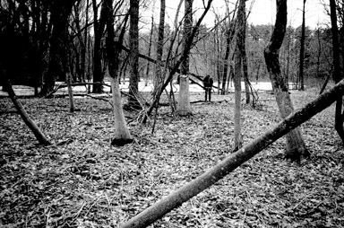
From about 24,000–31,000 ft (1.5 mi) along the longitudinal profile (fig. 9), the general character of channel substrate in the Wolf River changes from mainly sand to cobble, gravel, and sand. The channel is 200–250 ft wide through this reach. Transect T9 is at 29,970 ft along the longitudinal profile and is about 3,000 ft downstream from Keshena Falls (fig. 9). This transect bisects an island and is in the widest expanse of flood plain (about 900 ft) along the entire 6-mi study reach (fig. 20).
The main channel and side channel at transect T9 are characterized by gravel, cobble, and boulder (fig. 20). The island between the main and side channel is wooded and composed of about 4 ft of loam or sand over gravel. The elevation of the island is in the range of the stage of a 2- to 5-year flood. The area of flood plain between the side and flood channel is at the same elevation and also wooded. Tree trunks in this zone are scarred from ice jams and are evidence that water levels reach 5 ft above the flood-plain surface from ice-jam-related winter floods (fig. 21). The winter floods inundate the entire flood plain along the transect and are different than precipitation- or snowmelt-generated floods in that they cause ice damage and may be of longer duration. The ice-jam floods have occurred only after the failure of the Keshena Falls Dam. The jams occur at about 20,000 ft along the longitudinal profile and are caused by the flattening of the water-surface slope at this location (fig. 9). The slope flattens at this location because of impoundment effects from the Balsam Row Dam. Ice that formerly built up behind the Keshena Falls Dam before it failed now is able to move downstream and accumulates in the area where the slope flattens.
The core and survey data from transect T9 and GLO notes indicate that the river has narrowed and incised at this location since the late 1800s (fig. 20). Transect T9 bisects the section line between sections 22 and 27, T. 28 N., R. 15 E. The 1999 channel was about 200 ft wide, including the island. In 1891, the east side of the river was recorded in the GLO notes as being a perpendicular bluff 75 ft above the river; the channel width was 685 ft, and the right bank was 70 ft west of its location in 1999 (fig. 20). There is no mention of islands in the GLO notes. At T9-2, large wood pieces 2.5 ft below the flood-plain surface had calibrated radiocarbon ages of 1740±70, evidence of post-settlement burial of the west part of the channel. Based on depth of gravel in cores T9-1, T9-2, T9-2.5, T9-2.3 and T9-2.8, the 1891 channel bottom was about 2 ft higher than the 1999 channel bottom. Transect T9 is about 2,000 ft downstream from Keshena Falls and immediately downstream from a bedrock outcrop (fig. 9). The channel at this location was likely in a downstream scour zone related to locally decreased sediment inputs, a result of sediment capture behind the Keshena Falls Dam while it was in operation. Also, loggers may have dynamited and deepened the channel at this location for easier passage of logs.
The higher area of flood plain west of core T9-3.5 represents the pre-1891 flood-plain surface (fig. 20). Gravel was found in cores T9-5 and T9-5.5 at the same elevation as in the 1891 channel (as inferred from cores T9-1 through T9-3), likely indicating that the pre-1891 channel migrated laterally but did not aggrade or incise. The 1999 thalweg is deeper than any gravel related to relict channels, indicating that incision during the last 100 years probably relates to logging, log drives, and (or) the Keshena Falls Dam construction. GLO notes indicated that the area surrounding the transect had been clear-cut before the survey and that in 1891 the vegetation consisted of a dense growth of alder along the right bank and aspen brush and birch in the flood plain and upland, with scatterings of white and Norway pine.
In summary, channel characteristics in the rocky reach are not affected by the Balsam Row Dam but are likely affected by a combination of historical human disturbance related to logging and log drives and downstream scour resulting from the Keshena Falls Dam. The river width at transect T9 narrowed considerably after 1891 and incised 2 ft. Part of the 1891 channel is filled with about 2 ft of organic-rich loam. The exact cause for the narrowing is not known. Ice jams cause flooding in the wide flood plain at T9. The effects of this flooding on flood-plain vegetation are not known.
Selected intervals from six cores from transect T2, T4, T7, and T9 were analyzed for minor- and trace-element concentrations (tables 3 and 6). Detailed profiles of minor and trace elements for impounded sediment were constructed from 12 samples from core T2-1 over a range in depth that included one pre-dam sample (fig. 22). Samples of backwater sediment from the east side of transect T4 (cores T4-7 and T4-9) (fig. 16) and the west side of transect T7 (core T7-2) (fig. 19) were analyzed, as well as island sediment from transect T7 (core T7-12) (fig. 19) and flood-plain sediment from transect T9 (core T9-2) (fig. 20). All sediment sampled was deposited after the 1870s, based on interpretations of sedimentation rates and sediment sources discussed in the previous section. Concentrations of lead, mercury, and zinc were low in samples from 1.1 to 1.2 ft in core T4-7, from 0.5 to 0.8 ft in core T7-2, and from 1.9 to 2.8 ft in core T9-2. Samples from core T7-2 and T9-2 generally were more coarse-grained than other samples from backwater and impounded areas, which partially explains the low concentrations (table 6); many trace elements have an affinity for clay minerals and organic matter and are found in higher concentrations in organic-rich, fine-grained sediment compared to coarse-grained sediment (Horowitz, 1991).
[USGS, U.S. Geological Survey; ft, feet; pct, percent; µg/g, micrograms per gram; na, not analyzed; <, less than. Threshold and probable effect concentrations are from MacDonald and others (2000). Concentrations above the threshold effect concentration are listed in bold.]
| Core number | USGS site number | Interval top (ft) | Interval bottom (ft) | Date collected | Calcium (pct) | Magnesium (pct) | Potassium (pct) | Sodium (pct) | Sulfur (pct) | Phosphorus (pct) |
|---|---|---|---|---|---|---|---|---|---|---|
| T2-1 | 445022088373500 | 0.0 | 0.25 | 2/17/1999 | 2.0 | 0.77 | 0.97 | 0.51 | 0.44 | 0.19 |
| T2-1 | 445022088373500 | .75 | 1.0 | 2/17/1999 | 1.9 | .74 | 1.0 | .51 | .41 | .17 |
| T2-1 | 445022088373500 | 1.5 | 1.75 | 2/17/1999 | 1.9 | .71 | .96 | .48 | .48 | .15 |
| T2-1 | 445022088373500 | 2.0 | 2.25 | 2/17/1999 | 1.9 | .74 | 1.0 | .50 | .50 | .18 |
| T2-1 | 445022088373500 | 2.25 | 2.5 | 2/17/1999 | 1.8 | .76 | 1.0 | .50 | .52 | .16 |
| T2-1 | 445022088373500 | 2.25 | 2.5 | 2/17/1999 | 1.7 | .69 | .95 | .45 | .51 | .14 |
| T2-1 | 445022088373500 | 2.5 | 2.75 | 2/17/1999 | 1.9 | .76 | 1.1 | .52 | .55 | .13 |
| T2-1 | 445022088373500 | 3.0 | 3.25 | 2/17/1999 | 1.8 | .72 | 1.1 | .51 | .56 | .12 |
| T2-1 | 445022088373500 | 3.25 | 3.5 | 2/17/1999 | 1.7 | .68 | 1.0 | .48 | .49 | .12 |
| T2-1 | 445022088373500 | 3.5 | 3.75 | 2/17/1999 | 1.6 | .68 | 1.0 | .50 | .47 | .12 |
| T2-1 | 445022088373500 | 4.5 | 4.75 | 2/17/1999 | 1.7 | .71 | 1.0 | .48 | .49 | .13 |
| T2-1 | 445022088373500 | 5.75 | 6.0 | 2/17/1999 | 1.7 | .68 | 1.0 | .46 | .51 | .13 |
| T2-1 | 445022088373500 | 7.0 | 7.25 | 2/17/1999 | 1.5 | .60 | .91 | .42 | .50 | .11 |
| T4-7 | 445126088383400 | .0 | .1 | 6/21/1999 | 2.3 | .59 | .66 | .31 | 1.1 | .10 |
| T4-7 | 445126088383400 | 1.1 | 1.2 | 6/21/1999 | 1.6 | .52 | 1.0 | .53 | .39 | .06 |
| T4-9 | 445125088383400 | .0 | .1 | 6/21/1999 | 2.0 | .79 | 1.2 | .57 | .36 | .06 |
| T4-9 | 445125088383400 | .1 | .25 | 6/21/1999 | 1.9 | .76 | 1.2 | .58 | .41 | .07 |
| T7-2 | 445244088380500 | .0 | .1 | 6/23/1999 | 1.7 | .59 | 1.1 | .53 | .38 | .10 |
| T7-2 | 445244088380500 | .5 | .6 | 6/23/1999 | 1.5 | .75 | 1.6 | .77 | .06 | .04 |
| T7-2 | 445244088380500 | .7 | .8 | 6/23/1999 | 1.5 | .82 | 1.5 | .70 | <.05 | .03 |
| T7-12 | 445242088380500 | .0 | .2 | 6/23/1999 | 1.8 | .56 | .96 | .47 | .25 | .17 |
| T7-12 | 445242088380500 | .7 | 1.0 | 6/23/1999 | 1.6 | .59 | 1.5 | .74 | .13 | .12 |
| T7-12 | 445242088380500 | 1.8 | 2.0 | 6/23/1999 | 1.7 | .84 | 1.7 | .80 | .12 | .07 |
| T9-2 | 445306088391900 | .0 | .2 | 6/11/1999 | 1.3 | .40 | 1.3 | .66 | .14 | .08 |
| T9-2 | 445306088391900 | .5 | .7 | 6/11/1999 | 1.4 | .48 | 1.6 | .80 | .11 | .09 |
| T9-2 | 445306088391900 | 1.2 | 1.4 | 6/11/1999 | 1.3 | .57 | 1.7 | .82 | .06 | .09 |
| T9-2 | 445306088391900 | 1.9 | 2.1 | 6/11/1999 | 1.4 | .51 | 1.6 | .77 | .21 | .07 |
| T9-2 | 445306088391900 | 2.6 | 2.8 | 6/11/1999 | 1.3 | .50 | 1.5 | .79 | .12 | .04 |
| Threshold effect concentration | na | na | na | na | na | na | ||||
| Probable effect concentration | na | na | na | na | na | na | ||||
| Wolf River surficial sediment, 1996–98 (Garn and others, 2001) | 1.8–1.9 | 0.66–0.73 | 0.79–0.98 | 0.37–0.56 | 0.29–0.37 | 0.19–0.23 | ||||
| Core number | Interval top (ft) | Interval bottom (ft) | Inorganic carbon (pct) | Total carbon (pct) | Organic carbon (pct) | Aluminum (pct) | Arsenic ( µ g/g) | Barium ( µ g/g) | Cadmium ( µ g/g) | Chromium ( µ g/g) |
|---|---|---|---|---|---|---|---|---|---|---|
| T2-1 | 0.0 | 0.25 | 0.20 | 18.0 | 18.0 | 3.0 | 9.6 | 280 | 0.9 | 67 |
| T2-1 | .75 | 1.0 | .20 | 18.0 | 17.5 | 3.0 | 9.1 | 300 | 1.0 | 66 |
| T2-1 | 1.5 | 1.75 | .24 | 17.0 | 17.2 | 2.9 | 8.4 | 270 | 1.0 | 63 |
| T2-1 | 2.0 | 2.25 | .17 | 17.0 | 17.0 | 3.1 | 9.0 | 280 | 1.2 | 69 |
| T2-1 | 2.25 | 2.5 | .17 | 17.0 | 17.0 | 3.2 | 8.8 | 290 | 1.3 | 69 |
| T2-1 | 2.25 | 2.5 | .01 | 16.9 | 16.9 | 2.8 | 8.6 | 290 | 1.2 | 68 |
| T2-1 | 2.5 | 2.75 | .18 | 17.0 | 16.7 | 3.2 | 9.0 | 290 | 1.3 | 69 |
| T2-1 | 3.0 | 3.25 | .18 | 17.0 | 16.6 | 3.2 | 9.1 | 300 | 1.4 | 68 |
| T2-1 | 3.25 | 3.5 | .14 | 17.0 | 16.5 | 3.0 | 9.1 | 300 | 1.3 | 66 |
| T2-1 | 3.5 | 3.75 | .15 | 16.0 | 15.6 | 3.0 | 8.4 | 280 | 1.2 | 62 |
| T2-1 | 4.5 | 4.75 | .12 | 16.0 | 16.0 | 3.2 | 8.6 | 270 | 1.3 | 67 |
| T2-1 | 5.75 | 6.0 | .12 | 16.0 | 16.1 | 3.1 | 9.0 | 300 | 1.3 | 67 |
| T2-1 | 7.0 | 7.25 | .11 | 16.0 | 16.4 | 2.6 | 7.7 | 270 | 1.2 | 65 |
| T4-7 | .0 | .1 | .10 | 28.0 | 28.0 | 1.9 | 7.8 | 200 | .8 | 40 |
| T4-7 | 1.1 | 1.2 | .02 | 17.0 | 17.0 | 2.8 | 4.3 | 300 | .4 | 77 |
| T4-9 | .0 | .1 | .30 | 16.0 | 16.0 | 2.7 | 5.5 | 330 | .7 | 46 |
| T4-9 | .1 | .25 | .20 | 14.0 | 14.0 | 3.1 | 6.7 | 340 | .8 | 55 |
| T7-2 | .0 | .1 | .15 | 14.0 | 13.0 | 3.1 | 8.0 | 380 | .8 | 56 |
| T7-2 | .5 | .6 | .28 | 5.0 | 4.7 | 3.4 | 2.2 | 410 | .1 | 36 |
| T7-2 | .7 | .8 | .43 | 3.2 | 2.7 | 3.0 | 2.7 | 370 | .1 | 30 |
| T7-12 | .0 | .2 | .13 | 16.0 | 16.0 | 2.6 | 9.5 | 340 | .7 | 56 |
| T7-12 | .7 | 1.0 | .13 | 8.1 | 8.0 | 3.4 | 10.0 | 430 | .7 | 50 |
| T7-12 | 1.8 | 2.0 | .28 | 4.3 | 4.0 | 3.6 | 4.4 | 450 | .3 | 47 |
| T9-2 | .0 | .2 | .06 | 9.2 | 9.2 | 2.8 | 6.3 | 370 | .3 | 37 |
| T9-2 | .5 | .7 | .04 | 6.4 | 6.4 | 3.6 | 8.3 | 450 | .6 | 49 |
| T9-2 | 1.2 | 1.4 | .05 | 3.9 | 3.8 | 4.1 | 14.0 | 500 | .6 | 55 |
| T9-2 | 1.9 | 2.1 | .02 | 8.7 | 8.7 | 3.6 | 4.4 | 390 | .1 | 50 |
| T9-2 | 2.6 | 2.8 | .16 | 7.1 | 7.0 | 3.0 | 2.6 | 390 | .1 | 34 |
| Threshold effect concentration | na | na | na | na | 9.79 | na | 0.99 | 43.4 | ||
| Probable effect concentration | na | na | na | na | 33.0 | na | 4.98 | 111 | ||
| Wolf River surficial sediment, 1996–98 | 0.26–0.31 | 11.9–13.8 | 11.6–13.5 | 2.3–2.8 | 11.0–17.0 | 340–350 | 0.56–0.70 | 45–59 | ||
| Core number | Interval top (ft) | Interval bottom (ft) | Copper ( µ g/g) | Iron ( µ g/g) | Lead ( µ g/g) | Manganese ( µ g/g) | Mercury ( µ g/g) | Nickel ( µ g/g) | Selenium ( µ g/g) | Silver ( µ g/g) |
|---|---|---|---|---|---|---|---|---|---|---|
| T2-1 | 0.0 | 0.25 | 20 | 2.7 | 28 | 1,400 | 0.14 | 11 | 2.6 | 0.5 |
| T2-1 | .75 | 1.0 | 20 | 2.6 | 32 | 1,200 | .15 | 12 | 2.6 | .4 |
| T2-1 | 1.5 | 1.75 | 20 | 2.4 | 37 | 860 | .14 | 11 | 2.6 | .3 |
| T2-1 | 2.0 | 2.25 | 22 | 2.7 | 47 | 860 | .15 | 13 | 2.6 | .2 |
| T2-1 | 2.25 | 2.5 | 23 | 2.6 | 55 | 760 | .16 | 13 | 2.7 | .2 |
| T2-1 | 2.25 | 2.5 | 21 | 2.4 | 52 | 670 | .17 | 12 | 2.7 | .2 |
| T2-1 | 2.5 | 2.75 | 23 | 2.5 | 56 | 680 | .15 | 13 | 2.7 | .2 |
| T2-1 | 3.0 | 3.25 | 22 | 2.5 | 65 | 660 | .16 | 13 | 2.6 | .2 |
| T2-1 | 3.25 | 3.5 | 21 | 2.3 | 71 | 600 | .17 | 12 | 2.7 | .2 |
| T2-1 | 3.5 | 3.75 | 20 | 2.1 | 59 | 580 | .17 | 11 | 2.6 | .1 |
| T2-1 | 4.5 | 4.75 | 21 | 2.4 | 49 | 680 | .15 | 12 | 2.6 | <.1 |
| T2-1 | 5.75 | 6.0 | 22 | 2.5 | 49 | 670 | .18 | 13 | 2.7 | .2 |
| T2-1 | 7.0 | 7.25 | 20 | 2.1 | 43 | 560 | .17 | 11 | 2.6 | .1 |
| T4-7 | .0 | .1 | 16 | 1.3 | 26 | 140 | .19 | 8.0 | 2.3 | .7 |
| T4-7 | 1.1 | 1.2 | 17 | 1.1 | 5.0 | 170 | .09 | 10 | 2.9 | .2 |
| T4-9 | .0 | .1 | 16 | 1.7 | 18 | 270 | .15 | 10 | 1.7 | .3 |
| T4-9 | .1 | .25 | 28 | 1.8 | 27 | 270 | .17 | 11 | 1.8 | .3 |
| T7-2 | .0 | .1 | 40 | 2.3 | 27 | 1,100 | .28 | 12 | 1.9 | 2.3 |
| T7-2 | .5 | .6 | 12 | 1.8 | 9.0 | 470 | .03 | 10 | .8 | .5 |
| T7-2 | .7 | .8 | 10 | 1.4 | 7.0 | 350 | .03 | 9.0 | .4 | .2 |
| T7-12 | .0 | .2 | 20 | 2.6 | 19 | 2,800 | .16 | 11 | 2.0 | .5 |
| T7-12 | .7 | 1.0 | 17 | 2.8 | 26 | 2,400 | .11 | 11 | 1.6 | .6 |
| T7-12 | 1.8 | 2.0 | 16 | 2.3 | 15 | 530 | .07 | 12 | .9 | .5 |
| T9-2 | .0 | .2 | 11 | 2.0 | 14 | 1,700 | .10 | 8.0 | 1.3 | .3 |
| T9-2 | .5 | .7 | 15 | 2.7 | 29 | 1,900 | .13 | 11 | 1.6 | .5 |
| T9-2 | 1.2 | 1.4 | 16 | 3.5 | 17 | 4,300 | .13 | 14 | 1.8 | .5 |
| T9-2 | 1.9 | 2.1 | 17 | 1.7 | 9.0 | 540 | .09 | 11 | 1.6 | .5 |
| T9-2 | 2.6 | 2.8 | 9.0 | 1.0 | 7.0 | 270 | .07 | 7.0 | 1.1 | .2 |
| Threshold effect concentration | 31.6 | na | 35.8 | na | 0.18 | 22.7 | na | na | ||
| Probable effect concentration | 149 | na | 128 | na | 1.06 | 48.6 | na | na | ||
| Wolf River surficial sediment, 1996–98 | 13.8–18.0 | 2.7–3.0 | 23.0–26.0 | 2,800–3,500 | 0.08–0.1 | 9.6–12.0 | 1.6–1.8 | 0.20–0.44 | ||
| Core number | Interval top (ft) | Interval bottom (ft) | Strontium ( µ g/g) | Titanium ( µ g/g) | Uranium ( µ g/g) | Zinc ( µ g/g) | Sand (pct) | Silt (pct) | Clay (pct) |
|---|---|---|---|---|---|---|---|---|---|
| T2-1 | 0.0 | 0.25 | 76 | 0.15 | 4.6 | 110 | 8.9 | 39.5 | 51.6 |
| T2-1 | .75 | 1.0 | 79 | .16 | 5.3 | 120 | 9.0 | 41.4 | 49.6 |
| T2-1 | 1.5 | 1.75 | 71 | .16 | 5.4 | 120 | 5.3 | 58.3 | 36.4 |
| T2-1 | 2.0 | 2.25 | 76 | .16 | 5.6 | 140 | 9.4 | 39.7 | 50.9 |
| T2-1 | 2.25 | 2.5 | 77 | .16 | 6.5 | 140 | 6.8 | 37.2 | 56.0 |
| T2-1 | 2.25 | 2.5 | 72 | .19 | 6.4 | 140 | na | na | na |
| T2-1 | 2.5 | 2.75 | 79 | .16 | 6.4 | 150 | 4.2 | 46.0 | 49.8 |
| T2-1 | 3.0 | 3.25 | 78 | .16 | 6.0 | 150 | 3.9 | 38.4 | 57.7 |
| T2-1 | 3.25 | 3.5 | 75 | .20 | 6.4 | 150 | 4.0 | 39.4 | 56.6 |
| T2-1 | 3.5 | 3.75 | 73 | .17 | 5.6 | 140 | na | na | na |
| T2-1 | 4.5 | 4.75 | 74 | .16 | 5.9 | 140 | 3.2 | 48.9 | 47.9 |
| T2-1 | 5.75 | 6.0 | 76 | .18 | 6.1 | 150 | 4.5 | 43.8 | 51.7 |
| T2-1 | 7.0 | 7.25 | 66 | .18 | 5.5 | 130 | 74.3 | 14.9 | 10.8 |
| T4-7 | .0 | .1 | 52 | .12 | 12 | 53 | 12.5 | 44.0 | 43.5 |
| T4-7 | 1.1 | 1.2 | 71 | .19 | 4.4 | 74 | 43.8 | 28.5 | 27.7 |
| T4-9 | .0 | .1 | 79 | .19 | 5.4 | 90 | 67.7 | 17.3 | 15.0 |
| T4-9 | .1 | .25 | 79 | .18 | 5.0 | 120 | na | na | na |
| T7-2 | .0 | .1 | 75 | .21 | 5.6 | 100 | 29.3 | 41.8 | 28.9 |
| T7-2 | .5 | .6 | 95 | .22 | 2.6 | 48 | 77.8 | 17.5 | 4.7 |
| T7-2 | .7 | .8 | 83 | .18 | 2.4 | 40 | 95.9 | 2.8 | 1.3 |
| T7-12 | .0 | .2 | 76 | .17 | 5.4 | 110 | 44.6 | 33.7 | 21.7 |
| T7-12 | .7 | 1.0 | 98 | .23 | 4.3 | 98 | 79.1 | 12.6 | 8.3 |
| T7-12 | 1.8 | 2.0 | 100 | .25 | 3.8 | 71 | 78.1 | 15.8 | 6.1 |
| T9-2 | .0 | .2 | 82 | .18 | 4.9 | 64 | 85.1 | 9.8 | 5.1 |
| T9-2 | .5 | .7 | 98 | .24 | 5.0 | 91 | 80.1 | 14.0 | 5.9 |
| T9-2 | 1.2 | 1.4 | 100 | .27 | 5.1 | 83 | 76.1 | 17.6 | 6.3 |
| T9-2 | 1.9 | 2.1 | 100 | .25 | 9.0 | 50 | 77.3 | 19.2 | 3.5 |
| T9-2 | 2.6 | 2.8 | 89 | .17 | 5.5 | 43 | 86.7 | 7.4 | 5.9 |
| Threshold effect concentration | na | na | na | 121 | na | na | na | ||
| Probable effect concentration | na | na | na | 459 | na | na | na | ||
| Wolf River surficial sediment, 1996–98 | 70–81 | 0.14–0.20 | 2.4–3.6 | 82–89 | na | na | na | ||
The sample from T4-7 in the 1.0–1.2 ft interval was a mix of sand, silt, and clay in similar percentages as the surficial sample (0–0.2 ft) from core T7-12, and both samples had similar concentrations of organic carbon (table 6). However, concentrations of arsenic, cadmium, lead, and mercury in the surficial T7-12 sample are near or more than twice those in the T4-7 sample from 1.0 to 1.2 ft. Concentrations of chromium, copper, and nickel were similar in the two samples. This similarity suggests, as does the sedimentation history presented earlier, that the sand loam in core T4-7 between the peat layer most likely was deposited about the time of logging or log drives. This sample is indicative of background concentrations (pre-European settlement) for relatively coarse-grained fluvial deposits (44 percent sand, 29 percent silt, and 28 percent clay) with high amounts of organic matter (17 percent organic carbon) for the Wolf River.
Minor- and trace-element concentration profiles from core T2-1 from the Balsam Row Dam impoundment are representative of fine-grained deposits (generally greater than 50 percent clay) with relatively high amounts of organic matter (15.6–18.0 percent organic carbon) (fig. 22). Profiles of cadmium, lead, and zinc are similar, with peak concentrations at about 3.2 ft (late 1960s), decreasing concentrations upcore from 3.2 to 1.8 ft (1970–90), and concentrations in the top 1 ft (1990s) less than the pre-1960 concentrations. The range of concentrations in the profiles for these elements is greater than within- sample variability, as evidenced by low variability in concentrations for these elements in the duplicate sample for core interval 2.25–2.5 (table 6).
Subsurface peaks in lead concentrations also have been dated from the 1960s to early 1970s in other lakes and impoundments (Callender and Van Metre, 1997; Fitzpatrick and others, 2003). Decreasing concentrations of lead in the late 1970s were expected because of the reduction of air emissions of particulate lead after the passage of the Clean Air Act in 1970. Lead concentrations in the top of core T2-1 are lower than concentrations in the pre-dam sample; this may be due to dilution by higher percentages of organic matter at the top of the core (fig. 14C). This pattern also was seen in a sediment core from a bay of Lac Courte Oreilles, in northwestern Wisconsin (Fitzpatrick and others, 2003).
Cadmium and zinc concentrations may reflect historical regional air emissions from smelters in northern Wisconsin. However, the elevated concentrations are in the same range of the core where physical characteristics and radiometric dating indicate input of sediment from the Keshena Dam impoundment. Perhaps sediment stored behind the Keshena Dam historically had higher concentrations of atmospherically or watershed-derived trace elements than more locally derived sediment that would have been deposited in the Balsam Row Dam Impoundment when the Keshena Dam was functioning.
Aluminum and titanium are considered conservative elements that are associated with the mineral component of the sediment, and the profiles for these elements for core T2-1 (fig. 22D) show unchanging concentrations along the entire length of core. There is no evidence in the profile for a change in conservative element concentrations from input of sediment from the Keshena Falls Dam Impoundment after the dam failure.
Concentrations of arsenic, cadmium, chromium, copper, lead, mercury, nickel, and zinc in sediment from all sampled locations and core intervals were all below consensus-based probable effect concentrations (PEC), above which harmful effects on aquatic life are likely to be observed (table 6) (MacDonald and others, 2000). Two samples from flood-plain sediment were above the consensus-based threshold effect concentration (TEC) for arsenic (MacDonald and others, 2000). (No harmful effects on aquatic life are expected for concentrations below the TEC.) Only samples from the impoundment core T2-1 were above the TEC for cadmium, lead, and zinc. Chromium concentrations were generally above the TEC from all deposition zones except for older sediment deposited before European settlement or during logging or log drives. Only one sample from surficial backwater sediment at transect T7 had a copper concentration above the TEC. The highest mercury concentration (slightly above the TEC) was from surficial backwater sediment at transect T7; one sample of surficial sediment at T4 also had a mercury concentration just above the TEC. Nickel concentrations in all samples were below the TEC.
Concentrations of minor and trace elements are similar to concentrations from sieved surficial sediment collected during 1996–98 near the Fairground Road Bridge (USGS identification number 04077100, fig. 1) at about 24,000 ft on the longitudinal profile (fig. 9, table 6) (Garn and others, 2001). Concentrations also were in the range of sieved surficial-sediment concentrations found by Scudder and others (1997) for western tributaries to Lake Michigan. However, arsenic, mercury, and selenium concentrations in Wolf River sediment from the impoundment were greater than the national median, and cadmium and lead concentrations were greater than the 75th percentile based on sieved sediment concentrations from 541 streams across the Nation (Rice, 1999). Arsenic and selenium concentrations most likely reflect contributions from bedrock sources. Mercury concentrations reflect contributions from wetlands in the watershed.
In summary, minor- and trace-element concentrations in sediment from depositional areas in impoundment, backwater, and flood-plain environments generally reflect background conditions as influenced by watershed geology and historical inputs from regional and local atmospheric deposition. All samples had concentrations below the PEC. Concentrations of cadmium, chromium, lead, and zinc were above the TEC in sediment from the Balsam Row impoundment. Some samples from backwater sediment from the sandy reach exceeded the TEC for copper and mercury.
The USGS and the Menominee Indian Tribe examined historical trends in streamflow, sedimentation, and sediment chemistry for the Wolf River as it flows through a 6-mi reach through the southern part of the Menominee Indian Reservation. This study was done to determine the upstream effects of the Balsam Row Dam on channel characteristics of the Wolf River and to distinguish long-term (from about 1850–1999) changes in streamflow, sedimentation, and sediment chemistry from land cover or climate changes.
Results from trend analyses of historical streamflow and precipitation data indicate that annual flood peaks decreased during 1907–49 but increased during 1950–96; this pattern likely reflects mainly changes in precipitation (upper air circulation patterns) for both pre- and post-1950 and possibly forest regrowth during 1907–49. Mean monthly streamflow during 1912–96 decreased for February and March but increased for June and July. These trends indicate that spring snowmelt is occurring earlier in the spring. Decreases in early summer flows also may be affected by increased evapotranspiration from forest regrowth.
Results from analysis of sediment cores along nine valley transects indicate that an increase in water-surface elevation of 15 ft associated with Balsam Row Dam has caused changes in channel conditions for about 4.3 mi upstream. The Balsam Row impoundment extends for 1.8 mi and contains up to 10 ft of silty clay. The impoundment has lost much of its storage capacity. Historical average linear sedimentation rates in the impoundment were similar during 1927–63 (0.09 ft/y) and 1963–1999 (0.10 ft/y). The average mass sedimentation rate during 1927–63 is 1.15 lb/ft2/y, slightly higher than the average mass sedimentation rate during 1963–99 of 1.04 lb/ft2/y. However, sedimentation in the impoundment during 1963–99 has been episodic and associated with large floods, especially the record flood in 1973 that occurred one year after the Keshena Falls Dam failure.
Sand deposition is common in the Wolf River channel upstream from the impounded reach for 2.5 mi. Sand in the channel overlies gravel substrate and abundant woody debris assumed to be associated with logging and log drives in the late 1800s. Most of the sand deposition can be associated with slope changes in the water surface from the Balsam Row impoundment, but some sand deposition may also may have been caused by logging, log drives, and the failure of the Keshena Falls Dam.
In the upstream 1.5-mi part of the studied reach, the substrate is mainly rocky. About 2,000 ft downstream from Keshena Falls, the channel has narrowed and incised since the 1890s. The narrowing and incision at this location were likely related to human alterations associated with logging, log drives, or scour related to the Keshena Falls Dam.
Results from analyses of minor and trace elements from selected core samples indicate that concentrations generally reflect background conditions as affected by watershed geology and historical inputs from regional and local atmospheric deposition. All samples had concentrations below the PEC. Concentrations of cadmium, chromium, lead, and zinc were above the TEC in sediment from the Balsam Row impoundment. Backwater sediment from the sandy reach had some samples above the TEC for copper and mercury.
Douglas Cox, Heather Pyatskowit, and Jeremy Pyatskowit of the Menominee Indian Tribe, Environmental Services, were invaluable at providing field assistance for coring and surveying, and use of their boat was greatly appreciated. The author also is thankful to the landowners along the Balsam Row impoundment who gave access for the transect surveys, especially Clarence Neitzel, Stanley and Sandra Keonig, Len Pubanz, and the Menominee Logging Museum. James Rauman (USGS, Middleton, Wis.), Ty Sabin (formerly USGS, Middleton, Wis.) and Faye Blondin (formerly USGS, Middleton, Wis.) were indispensable for geoprobe coring in extremely cold, wet, remote, hilly, and wooded conditions.
Many thanks also are in order for the technical guidance received. John Attig (Wisconsin Geological and Natural History Survey, Madison, Wis.) gave guidance on glacial history. Professor James Knox (University of Wisconsin-Madison, Madison, Wis.) gave guidance on fluvial geomorphic processes. Ted Callender (USGS, Reston, Va.) gave guidance on sediment chemistry. Dale Robertson (USGS, Middleton, Wis.) assisted with trend analysis. William Krug (USGS, Middleton, Wis.) helped with streamflow data retrievals. Herbert Garn (USGS, Middleton, Wis.), Douglas Cox, and Kyle Juracek (USGS, Lawrence, Kans.) greatly improved the content of this report through their thorough technical reviews. Michael Eberle (USGS, Columbus, Ohio) did the editorial review. Manuscript illustrations and tables were made possible through Marie Peppler (USGS, Middleton, Wis.), Heather Schwar (formerly USGS, Middleton, Wis.), and Amanda Bell (USGS, Middleton, Wis.). Michelle Greenwood and Susan Jones (USGS, Middleton, Wis.) completed the final layouts.
American Society for Testing and Materials, 1992, Standard test method for laboratory determination of water (moisture) content of soil and rock: Philadelphia, Pa., Annual Book of ASTM Standards, Designation D2216-92, p. 177–180.
Arbogast, B.F., 1996, Analytical methods for the Mineral Resource Surveys Program: U.S. Geological Survey Open-File Report 96–525, 248 p.
Birkland, P.W., 1984, Soils and geomorphology: New York, Oxford University Press, 372 p.
Bowman, Sheridan, 1990, Radiocarbon dating—Interpreting the past: London, British Museum Publications, 64 p.
Briggs, P.H., and Meier, A.L., 1999, The determination of 42 elements in geological materials by inductively coupled plasma mass spectrometry: U.S. Geological Survey Open-File Report 99–166, 15 p.
Callender, E., and Van Metre, P.C., 1997, Reservoir sediment cores show U.S. lead declines: Environmental Science & Technology, v. 31, no. 9, p. 424–428.
Clayton, L., Attig, J.W., Mickelson, D.M., and Johnson, M.D., 1991 (revised 1992), Glaciation of Wisconsin: Wisconsin Geological and Natural History Survey Educational Series 36, 4 p.
Connor, M.R., 1978, Logging in northeastern Wisconsin—Some historic events in Wisconsin's logging industry: inpp Proceedings of the Third Annual Meeting, Forest History Association, University of Wisconsin, Madison, Wis.: p. 31–38.
Dean, W.E., Jr., 1974, Determination of carbonate and organic matter in calcareous sediments and sedimentary rock by loss on ignition—Comparison with other methods: Journal of Sedimentary Petrology, v. 44, p. 242–248.
Eichenlaub, Val, 1979, Weather and climate of the Great Lakes region: Notre Dame, Ind., University of Notre Dame Press, 335 p.
Fitzpatrick, F.A., 1993, Effects of historical clear-cut logging on streamflow of two northern Wisconsin Streams [Abs.]: Gorden Conference on Hydrologic, Geochemical, and Biological Processes in Forested Catchments, Aug. 1–6, 1993, Plymouth, N.H.
Fitzpatrick, F.A., Garrison, P.J., Fitzgerald, S.A., and Elder, J.F., 2003, Nutrient, trace-element, and ecological history of Musky Bay, Lac Courte Oreilles, Wisconsin, as inferred from sediment cores: U.S. Geological Survey Water-Resources Investigations Report 02–4225, 141 p.
Fitzpatrick, F.A., Knox, J.C., and Whitman, H.E., 1999, Effects of historical land-cover changes on flooding and sedimentation, North Fish Creek, Wisconsin: U.S. Geological Survey Water-Resources Investigations Report 99–4083, 12 p.
Fries, R.F., 1951, Empire in pine, the story of lumbering in Wisconsin, 1830–1900: Madison, Wis., State Historical Society of Wisconsin, 285 p.
Garn, H.S., Scudder, B.C., Richards, K.D., and Sullivan, D.J., 2001, Characteristics of water, sediment and benthic communities of the Wolf River, Menominee Indian Reservation, Wisconsin, water years 1986–98: U.S. Geological Survey Water-Resources Investigations Report 01–4019, 54 p.
Gebert, W.A., and Krug, W.R., 1996, Streamflow trends in Wisconsin's Driftless Area: Journal of the American Water Resources Association, v. 32, no. 4, p. 733–744.
Goldberg, E.D., 1963, Geochronology with 210Pb: Vienna, Austria, International Atomic Energy Agency, Proceedings from a Symposium on Radioactive Dating, p. 121–131.
Gundlach, H.F., Campbell, J.E., Huffman, T.J., Kowalski, W.L, Newbury, R.L., and Roberts, D.C., 1982, Soil Survey of Shawano County: U.S. Department of Agriculture, Soil Conservation Service [variable pagination].
Guy, H.P., 1969, Laboratory theory and methods for sediment analysis: U.S. Geological Survey Techniques of Water-Resources Investigations, book 5, chap. C1, 58 p.
HÅkanson, L., and Jansson, M., 1983, Principles of lake sedimentation: Caldwell, New Jersey, Blackburn Press, 316 p. (Reprinted 2002.)
Horowitz, A.J., 1991, A primer on sediment-trace element chemistry (2d ed.): Chelsea, Mich., Lewis Publishers, 136 p.
Iman, R.L., and Conover, W.J., 1983, A modern approach to statistics: New York, John Wiley and Sons, 497 p.
Juracek, K.E., 2004, Flood-related, organic-carbon anomalies as possible temporal markers in reservoir bottom sediments: Lake and Reservoir Management, v. 20, no. 4, p. 309–321.
Kalnicky, R.A., 1974, Climatic change since 1950: Annals of the Association of American Geographers, v. 64, p. 100–112.
Knox, J.C., Bartlein, P.J., Hirschboeck, K.K., and Muckenhirn, R.J., 1975, The response of floods and sediment yields to climate variation and land use in the upper Mississippi valley: Madison, Wis., Center for Geographic Analysis, University of Wisconsin, Institute of Environmental Studies Report 52, 76 p.
Krishnaswami, S., and Lal, D., 1978, Radionuclide limnochronology, in Lerman, A., ed., Lakes—Chemistry, geology, physics: New York, Springer-Verlag, p. 153–177.
Krishnaswami, S., Lal, D., Martin, J.M., and Meybeck, M., 1971, Geochronology of lake sediments: Earth and Planetary Science Letters, v. 11, p. 407–414.
Krohelski, J.T., Kammerer, P.A., and Conlon, T.D., 1994, Water resources of the Menominee Indian Reservation of Wisconsin: U.S. Geological Survey Water-Resources Investigations Report 93–4053, 54 p., 4 pls.
Libby, W.F., 1946, Atmospheric helium three and radiocarbon from cosmic radiation: Physical Review, v. 69, p. 671–672.
MacDonald, D.D., Ingersoll, C.D., and Berger, T.A., 2000, Development and evaluation of consensus-based sediment quality guidelines for freshwater ecosystems: Archive of the Environmental Contamination Toxicologists, v. 39, p. 20–31.
Menominee Tribal Enterprises, 1997, The Menominee forest-based sustainable development tradition: Menominee Tribal Enterprises, Unpublished Report, 23 p.
Milfred, C.J., Olson, G.W., and Hole, F.D., 1967, Soil resources and forest ecology of Menominee County, Wisconsin: Madison, Wis., University of Wisconsin, Geological and Natural History Survey, Soil Survey Division, Bulletin 85, Soil Series No. 60: 203 p., and 3 pl.
Mudrey, M.G., Brown, B.A., and Greenburg, J.K., 1982, Bedrock geology map of Wisconsin: University of Wisconsin-Extension, Wisconsin Geological and Natural History Survey, scale 1:1,000,000, 1 oversized sheet.
Munsell Color, 1975, Munsell soil color charts: Baltimore, Munsell Color Division of Kollmorgen Corp. [variable pagination].
Oehmcke, A.A., and Truax, W.C., 1964, The Wolf River: Wisconsin Academy Transactions, v. 53 (Part A), p. 9–20.
Olcott, P.G., 1968, Water resources of Wisconsin-Fox-Wolf River Basin: U.S. Geological Survey Hydrologic Investigations Atlas HA–321, 4 sheets, scale 1:1,000,000.
Olsson, I.U., 1986, Radiometric dating, in Berglund, B.E., ed., Handbook of Holocene palaeoecology and palaeohydrology: Chichester, U.K., John Wiley and Sons, p. 273–312.
Peters, C.A. (ed.), 1997, Environmental setting and implications for water quality in the Western Lake Michigan Drainages: U.S. Geological Survey Water-Resources Investigations Report 97–4196, 79 p.
Pirkey, K.D., and Glodt, S.R., 1998, Quality control at the U.S. Geological Survey National Water Quality Laboratory: U.S. Geological Survey Fact Sheet FS–026–98, 6 p.
Rayburg, S.C., 1999, Streamflow response to land use change and climate variation in the Prairie River watershed, north central Wisconsin: University of Wisconsin-Madison, Geography Dept., Master's thesis, 79 p.
Reese, H.M., Lillesand, T., Nagel, D.E., Stewart, J.S., Goldmann, R.A., Simmons, T.E., Chipman, J.W., and Tessar, P.A., 2002, Statewide land cover derived from multiseasonal Landstat TM data—A retrospective of the WISCLAND project: Remote Sensing of the Environment, v. 82, p. 224–237.
Retallick, G., 1985, Laboratory exercises in paleopedology: Eugene, Oreg., University of Oregon, course handout, 74 p.
Rice, K.C., 1999, Trace-element concentrations in streambed sediment across the conterminous United States: Environmental Science & Technology, v. 33, p. 2,499–2,504.
Robbins, J.A., 1978, Geochemical and geophysical applications of radioactive lead, in Nriagu, J.O., ed., The biogeochemistry of lead in the environment: Amsterdam, Elsevier/North-Holland, p. 285–393.
Sartz, R.S., 1972, Soil water depletion by a hardwood forest in southwestern Wisconsin: Soil Science Society of America Proceedings, v. 36, p. 961–964.
Scudder, B.C., Sullivan, D.J., Fitzpatrick, F.A., and Rheaume, S.J., 1997, Trace elements and synthetic organic compounds in biota and streambed sediment of the western Lake Michigan drainages, 1992–95: U.S. Geological Survey Water-Resources Investigations Report 97–4192, 34 p.
Soil Survey Staff, 1951, Soil survey manual: U.S. Department of Agriculture, Agricultural Handbook 18, 503 p.
Smith, L.S., 1908, The water powers of Wisconsin: Wisconsin Geological and Natural History Survey Bulletin 20, Economic Series, No. 13 [variable pagination].
Stuiver, M., and others, 1998, INTCAL98 radiocarbon age calibration: Radiocarbon, v. 40, no. 3, p. 1,041–1,083.
Talma, A.S., and Vogel, J.C., 1993, A simplified approach to calibrating C14 dates: Radiocarbon, v. 35, no. 2, p. 317–322.
U.S. Army Corps of Engineers, 1993, Alternatives for flood control and study plan formulation, ice jam flooding on the Wolf River at Keshena, Wisconsin: St. Paul, Minn., 17 p.
U.S. Army Corps of Engineers, 1995, Flood plain delineation study, phase 1, Wolf River, Menominee Indian Tribe of Wisconsin, Menominee Reservation, Wisconsin: Detroit, Mich. [variable pagination].
U.S. Department of Agriculture and the University of Wisconsin, 1961, Physical supplies of water, water uses, and water demands—Statewide and Wolf River Basin: Madison, Wis., University of Wisconsin Draft Phase Report 11, Contract 12-14-100-1010(43), p. 64–138.
U.S. Geological Survey, 1961, Surface water records of Wisconsin, 1961: 143 p.
Wendland, W.M., Vogel, J.L., and Changnon, S.A., Jr., 1985, Mean 1951–1980 temperature and precipitation for the North Central Region: Champaign, Ill., Illinois State Water Survey, NCRCC Paper 7, 30 p.
Wright, H.E., 1967, A square-rod piston sampler for lake sediments: Journal of Sedimentary Petrology, v. 37, p. 975–976.
| Accessibility FOIA Privacy Policies and Notices | |

|
|