The U.S. Environmental Protection Agency (USEPA) method detection limit (MDL) is described as the minimum concentration of a substance that can be measured and reported with 99-percent confidence that the analyte concentration is greater than zero (U.S. Environmental Protection Agency, 1997) and is based on the approach of Glaser and others (1981). The MDL protects against incorrectly reporting the presence of a compound at low concentrations in cases when noise and actual analyte signal may be indistinguishable. The MDL concentration does not imply accuracy or precision of the quantitative measurement.
Reporting a detection when there is no substance present is known as a “false positive.” The USEPA MDL is designed to control against false positives at the 99-percent confidence level in an ideal matrix. Reporting the detection of a substance at the MDL concentration in a blank sample or a sample that does not contain the analyte should be rare (less than or equal to 1 percent). Therefore, a signal that represents the presence of a substance in a sample at the MDL concentration is not likely to be false.
 |
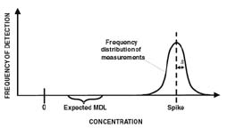
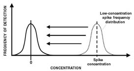
| Figure 1. The spike concentration in relation to the expected method detection limit (MDL). |
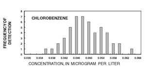
Collection of data points at this spike concentration produces a distribution of measured concentrations. As an example, figure 2 shows the resultant distribution (histogram) of measured concentrations of chlorobenzene obtained from 50 injections of a 0.05-microgram per liter (µg/L) spike using USGS method O-4127-96 (schedule 2020, Connor and others, 1998).
The frequency distribution of measured concentrations in the low-concentration spike that was used to determine the MDL is assumed in the USEPA procedure to have a normal distribution and is represented by the bell-shaped curve in figure 3. Also shown is one standard deviation (s) of this distribution.
 |
 |
|
Figure 2. Frequency distribution of measured concentrations of chlorobenzene spiked at 0.05 microgram per liter. |
Figure 3. Frequency distribution of measured concentrations of method detection limit (MDL) test samples spiked at 1 to 5 times the expected MDL concentration and showing one standard deviation (s). |
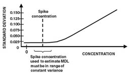
Another important assumption of the USEPA MDL calculation is that the frequency distribution of sequentially lower concentration replicate spikes, and thus the standard deviation of the distribution (not the percent relative standard deviation), will become constant at some low concentration and will remain constant down to zero concentration. The standard deviations calculated from low concentrations become similar because of the inability to adequately measure small differences in the diminishing signal. A representative graph of standard deviations for different spike concentrations is shown in figure 4. The USEPA procedure recommends that an iterative process be used to reduce the spike concentration to successively lower concentrations to help ensure that the region of practically constant standard deviation near the MDL has been reached.
Assuming constant standard deviation from the low-concentration spike down to zero, the frequency distribution of repetitive, low-concentration spikes is superimposed on zero concentration (analyte not present in samples) (fig. 5). This is the distribution that would be expected if measuring a signal from instrumental noise or actual unspiked analyte or both in a series of blank samples. Because it typically is impractical to measure noise in repetitive blank samples, the frequency distribution of the low-concentration spike is used as the hypothetical blank frequency distribution. The hypothetical blank measurements are used to calculate the concentration at which no more than 1 percent of the blank measurements will result in the reporting of a false positive.
 |
 |
|
Figure 4. Standard deviation in relation to concentration of analyte, showing a region of constant standard deviation at low concentrations. [MDL, method detection limit] |
Figure 5. The frequency distribution of the low-concentration spike measurements is centered on zero concentration to simulate the distribution expected for replicate blank measurements (analyte not present). |
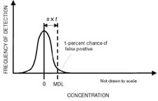
In summary, given the assumptions of constant standard deviation at low concentration, normal distribution, and minimal matrix interferences, the USEPA MDL is the concentration at which no more than 1 percent of the blank measurements result in a false positive detection (fig. 6). Therefore, detections at concentrations greater than or equal to the MDL concentration should be true detections 99 percent of the time. The USEPA MDL is calculated in equation 1:
 |
|
Figure 6. The U.S. Environmental Protection Agency’s method detection limit (MDL) is set at a concentration to provide a false positive rate of no more than 1 percent. [s, one standard deviation; t, Student’s t value at the 99-percent confidence level] |

Limitations of the USEPA MDL procedure include the assumptions of normal distribution and constant standard deviation over the low-concentration range from the spike concentration that is used to determine the MDL down to zero concentration. These and other limitations and considerations have been discussed in detail elsewhere, for example, Keith, 1992; Eaton, 1993; Gibbons, 1996; Gibbons and others, 1997a; Hall and Mills, 1997.
The MDL typically is determined by using a minimal number of spike replicates (n > 7) that are measured over a short time period; this provides only a narrow estimate of the overall method variation and, thus, the standard deviation (s). If performed in this manner, the USEPA procedure is especially inadequate for production laboratories where there are multiple sources of method variation, including multiple instruments, instrument calibrations, and instrument operators; and for methods that require preparation steps, there are multiple preparation events and staff. Occasionally, a laboratory may calculate a USEPA MDL that is so low that under routine analysis it produces a signal that cannot be reliably distinguished from instrument noise. This happens most often with single-instrument, single-calibration, and(or) single-operator tests that result in estimates of the standard deviation that are too small. In this case, the actual false positive probability at the USEPA MDL likely exceeds the desired 1-percent maximum. Consequently, the MDL needs to be determined by using routine conditions and procedures. This means conducting the determination over an extended time period by using all method instrumentation and as many variables as feasible to obtain a more accurate and realistic measurement of the standard deviation near the MDL.
Use by the National Water Quality Laboratory
In 1992, the NWQL began applying the USEPA procedure (U.S. Environmental Protection Agency, 1984, 1997 [Note: Revision 1.11 has remained unchanged since 1984]) for determining MDL’s for two methods developed for the National Water-Quality Assessment Program. These methods were for pesticides in water by C-18 solid-phase extraction with analysis by gas chromatography/mass spectrometry (NWQL analytical schedules 2001/2010; Zaugg and others, 1995) and pesticides in water by Carbopak-B solid-phase extraction with analysis by high performance liquid chromatography with diode array detection (schedules 2050/2051; Werner and others, 1996). For these methods, the reporting level was set equivalent to the MDL determined by using the USEPA procedure for all analytes in schedules 2001/2010 (Zaugg and others, 1995, table 9) and for 20 of the 41 analytes in schedules 2050/2051 (U.S. Geological Survey National Water Quality Laboratory Technical Memorandum 98.03A, 1997). The data-reporting conventions used for these methods were detailed in U.S. Geological Survey National Water Quality Laboratory Technical Memorandum 94.12 (1994). The USEPA procedure was chosen because it was viewed by the NWQL as being a “generally accepted” procedure for determining MDL’s; it is required by USEPA as a test of acceptable performance of analytical method detection capability for laboratories that use USEPA methods. Additionally, the USEPA MDL procedure is a statistically based approach that could be applied consistently across all NWQL methods.