This programmers guide provides an introduction to the programming in ModelMuse and describes tools that can be used to obtain a more complete description or to use for testing. ModelMuse is written in Object Pascal and can be compiled using Embarcadero Delphi XE. Among the introductions to Object Pascal are Shemitz (2002), Cantù (2003), and Calvert and others (2002). The website http://www.marcocantu.com/ contains useful guides that can be downloaded. Other useful resources include Thorpe (1997), and Konopka (1997).
One central class is TPhastModel. It stores a representation of the model. The grid for the model is stored in TCustomModel.PhastGrid or TCustomModel.ModflowGrid. The objects (TScreenObject) are stored in TPhastModel.ScreenObjects. For the purposes of reading or writing TScreenObjects to or from a stream, TPhastModel.ObjectList is used instead of TPhastModel.ScreenObjects. TPhastModel descends from TComponent and the usual component streaming methods are used to save the model to a file or read it from a file.
The grid used in ModelMuse is represented by TPhastGrid or TModflowGrid both of which descends from TCustomModelGrid. TPhastGrid.LayerElevations stores the layer boundaries for PHAST models. TModflowGrid.LayerElevations stores the layer boundaries for MODFLOW models. TCustomModelGrid.ColumnPositions and TCustomModelGrid.RowPositions store the column and row boundaries.
Distributed properties such as hydraulic conductivity are defined by TDataArray or one of its descendants such as TCustomPhastDataSet. TDataArray.DataType indentifies what sort of data is stored in a TDataArray. The data itself can be accessed through BooleanData, IntegerData, RealData, or StringData. An important method of TDataArray is Initialize which assigns values to the data in TDataArray. Data sets that allow PHAST-style interpolation (set TPhastInterpolationValues) are represented by TCustomPhastDataSet which descends from TDataArray.
Ordinary data sets are edited using TfrmDataSets. It also ensures that the user enters valid formulas for TDataArrays.
Boundary conditions in ModelMuse are also represented by descendants of TDataArray. However, boundary conditions are only defined at some locations and not at others so it would be wasteful of memory to use an array to store the data. Instead a T3DSparsePointerArray is used to store the data in either a TSparseArrayPhastInterpolationDataSet or a TCustomSparseDataSet. The difference is that the former allows for PHAST-style interpolation and the latter does not.
Boundary conditions can change with time so the TDataArrays used to represent boundary conditions are stored in descendents of TCustomTimeList. The most important method of TCustomTimeList is Initialize which creates all the TDataArrays needed to represent a particular boundary condition and sets the values for those TDataArrays. In PHAST models, this method is called from TPhastModel.InitializeTimes.
The objects are represented by TScreenObject which descends from TObserver. TScreenObject extends TObserver by adding properties to define boundary conditions and to allow PHAST-style interpolation with TCustomPhastDataSets. (See TPhastInterpolationValues.) The locations of the vertices in a TScreenObject are stored in TScreenObject.Points. TScreenObject.DataSets stores the TDataArrays that are affected by the TScreenObject and TScreenObject.DataSetFormulas stores the corresponding formulas for the TDataArrays.
TScreenObject are edited by TfrmScreenObjectProperties which is responsible for ensuring that the user enters valid formulas for the data sets and boundary conditions. When the user first creates a TScreenObject, TfrmScreenObjectProperties.GetData is called to read the data from the TScreenObject and display it. Once the user clicks the OK button, TfrmScreenObjectProperties.SetData is called to set the TScreenObject's properties. If the user wants to edit the properties of a TScreenObject later on, TfrmScreenObjectProperties.GetDataForMultipleScreenObjects is called (even if the user is only editing one TScreenObject). TfrmScreenObjectProperties.SetMultipleScreenObjectData is called when the user clicks the OK button.
The main form of ModelMuse is frmGoPhast which is a TfrmGoPhast. TfrmGoPhast descends from TUndoForm which allows commands encapsulated as TUndoItems to be undone and redone. TfrmGoPhast pvovides the main menu, the buttons, the status bar, three instances of TframeView, and a Tframe3DView to show a 3D view of the model.
Each instance of Tframe3DView shows either the top, front, or side view of the model. Most of the mouse interaction is handled through Tframe3DView. Typically, however, that interaction is delegated to a descendent of TCustomInteractiveTool. Most of the descendants are defined in InteractiveTools.
PHAST requires it spatial data to be entered in zones. TCustomPhastZone is a base class that defines much of the behavior for zones. Descendants of it define zones for particular types of data including boundary conditions. The individual zones are stored in descendants of TCustomZoneGroup. Some zones must define more than one data set. The data sets for a particular zone are defined in descendants of TCustomDataSets.
The input file for PHAST is generated with an ordinary procedure WritePhastInput.
TShapefileGeometryReader is used to read the geometry of Shapes from ESRI Shapefiles. Each Shape is stored in a TShapeObject. Similarly, TShapefileGeometryWriter is used to write the geometry of Shapes to an ESRI Shapefile.
Most of the cursors used in ModelMuse are defined in CursorsFoiledAgain. Six however are generated and modified using instances of TQRbwDynamicCursor. One of these instances is TfrmGoPhast.dcAddColCursor.
Each name reflects the function of the thing being named.
The names of types that are derived from Exception begin with a capital E.
The names of pointer types begin with a capital P.
The names of all other types begin with a capital T.
The names of all cursor constants begin with a lower case cr.
The names of all resource strings begin either with a lower case rs or with Str.
The names of members of ordinal types begin with one to four lower case letters that are an abbreviation of the name of the type. For example there is an ordinal type named TElevationCount. Its members are named ecZero, ecOne, and ecTwo. In this case ec is an abbreviation for ElevationCount.
The names of the fields of classes begin with a capital F except for components in the published section of forms or frames.
The names of fields that are components in the published section of forms or frames and which are also used in the source code begin with several lower case letters that are an abbreviation of the name of the type of the component.
The names of fields that are components in the published section of forms or frames and but which are not referenced in the source code may either follow the above convention or have their name left at their default name assigned by Delphi. For example, a label that is never referenced in the source code might have its name left at Label1.
The names of form classes (descendants of TForm) begin with Tfrm.
The names of form global variables are the same as the name of the form classes except that the initial T is removed.
Most form classes have two methods named GetData and SetData. GetData is used when the form is displayed to retrieve data from the model and display it in the form. SetData is used to modify the model with the data that the user has modified it in the form.
The names of components classes or units that have a high potential for use in other projects include the authors initials (RBW) near the beginning of the class name. (This helps minimize the chances of naming conflicts if others use the components or units.)
These conventions apply only to the source code written by the author of this report. Some of the source code used in ModelMuse was made publicly available on the Internet by its original authors and was adopted for use in ModelMuse. No attempt has been made to modify such source code to make it conform to these naming conventions.
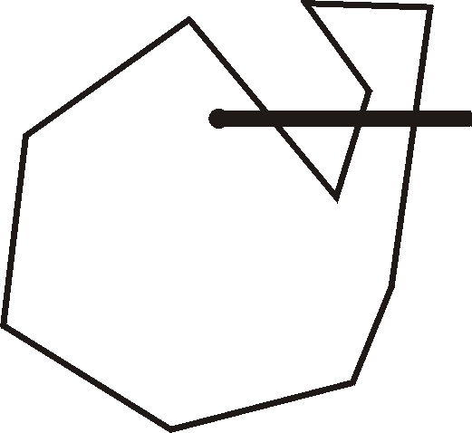
A well known algorithm for finding whether a point is inside a closed polygon is that of Shimrat (1980) . The same algorithm is also presented in O'Rourke (1998) with a more extensive explanation and several variations. The essence of the algorithm is to draw a horizontal line from the point in question to positive infinity and count the number of times this line intersects the outline of the polygon. If the number of times is odd, the point is inside the polygon. In the figure 2.1, for example, the algorithm determines that the point at the small black circle is inside the polygon because the line extending from it intersects the edge of the polygon three times.
|
| Figure 2.1, Polygon, point, and line illustrating algorithm. |
If a vertex of the polygon happens to lie directly on the line drawn from the point, it is only counted as an intersection with the segment for one of the two edges of the polygon of which it is a part.
For evaluating a single point, the algorithm is very efficient; the number of operations is proportional to the number of vertices in the polygon. However, if many points are to be tested with the same polygon, the efficiency can be improved in several ways.
If many of the tested points are likely to lie outside the polygon, one easy way to improve the algorithm is to construct a box surrounding the polygon (Figure 2.2). It will take, at most, four operations to test whether a point lies inside the box. If the point does lie inside the box, then the original test is performed to determine whether the point lies inside the polygon. Because many points are eliminated in the first test, the overall efficiency is improved.
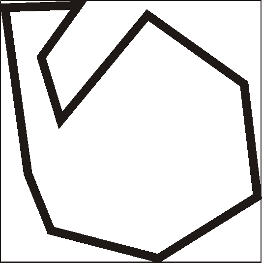 |
| Figure 2.2, Box around polygon. |
Another improvement can be implemented if the polygons are usually not very "jagged". A non-jagged polygon is one in which the positions of successive vertices along the edge of the polygon are positively correlated with one another; that is they tend to be close together. In figure 2.3, the polygon on the left is not jagged but the one on the right is jagged.
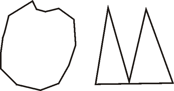 |
| Figure 2.3, Jagged and non-jagged polygons. |
The way the algorithm can be improved is to note that if one edge of the polygon is not to the left of the point of interest, its neighbors are unlikely to be to the left of it too. Thus, it makes sense to group as many edges of the polygon as possible together and see if the all can be eliminated in one step. In essence, a binary search tree is used to make the algorithm more efficient.
The first thing to do is to divide the polygon into two parts each of which consists of consecutive edges of the polygon. For each of these parts, compute the lowest and highest Y value and the largest X value. If the point of interest lies below the smallest Y, value, above the largest Y value or to the right of the largest X value, then all the edges in that group can be eliminated at once. If, the group of edges is not eliminated in this way, it can be subdivided in the same way as the original polygon and each of those parts can be tested in the same way. In this way a large number of sides of the polygon can be eliminated quickly and only a few will need to be tested with the original test. If the division into parts is only done once when the first point is tested and then the parts of the polygon are reused for subsequent points, testing the first point will be somewhat slower than the original algorithm but for each subsequent point, the number of operations will be proportional to the logarithm of the number of vertices. Of course, if the number of vertices in the polygon is small enough, the original algorithm is still more efficient but this is easy to handle.
This algorithm is illustrated in the figure 2.4. Figure 2.4A shows the point and polygon to be tested. The segments comprising the polygon have been numbered from 1 to 15. The polygon can be broken into two sections: segments 1-8 and segments 9-15. Because the minimum Y value in the first section is greater than the Y value of the point to be tested the first section can be eliminated from further consideration as shown in Figure 2.4B. The remaining section can also be divided into two sections: segments 9-12 and segments 13-15. However, neither of these sections can be eliminated immediately so both sections and split into two sections as shown in Figure 2.4C. Of the four sections shown in Figure 3, three can be eliminated either because the Y value of the point to be tested lies outside the range of the section or because the X value of the point to be tested is higher than the maximum X value of the section. This leaves one remaining section as illustrated in Figure 2.4D. The two segments would be tested to see if either or both lie to the right of the point to be tested. One of them does so the number of segments to the right of the point to be tested is one, which is an odd number. Therefore, the point is inside the original polygon.
 |
| Figure 2.4, Progressive steps in application of algorithm for determining if a point is inside a polygon. Arrows indicate where the polygon is being split. |
The number of comparisons that must be made is proportional to the log of the number of vertices in the polygon. The number of operations required to set up the polygon to be broken up into pieces is proportional to the number of vertices in the polygon times the log of the number of vertices. However, this step only needs to be done once for a polygon so if many points are being tested, there can be a net improvement in efficiency.
A polyline is a series of vertices that are connected by line segments. It is often of interest to know whether two polylines intersect each other. There are well known algorithms for testing whether two line segments intersect (O'Rourke (1998) ) so one easy way to test whether a pair of polylines intersect is to test each line segment in one line segment intersects any line segment in the other polyline. However, the time required to make this test is proportional to the product of the number of vertices in the two polylines. If the positions of successive vertices in the polyline are positively correlated with one another, then it is possible to use a more efficient algorithm. The technique is closely related to the methods used to speed up testing whether a point is inside a polygon. First, calculate the maximum and minimum X and Y coordinates of each polyline. It is easy to test whether the boxes constructed in this way overlap. If they don't, the polylines don't intersect either. If they do, the one of the polylines can be divided into two sections and the maximum and minimum X and Y coordinates of each section can be calculated. The two resulting polylines can each be recursively tested for intersection against the polyline that was not subdivided. At some point, if the polylines do intersect, each of the polylines that is being tested consists of only one line segment. At that point, the two segments can be tested for intersection in the usual manner. This process continues until two segments are found to intersect or all the segments have either been tested for intersection or have been eliminated.
The algorithm used to detect polylines with grid cells is simple. First, the coordinates of all the vertices in the polyline are rotated so that they are in a coordinate system in which the columns of the grid are perfectly vertical and the rows are perfectly horizontal. Then, a pair of binary searches through the rows and columns is used to determine which grid cell, if any, contains each vertex of the polyline (Figure 2.5, A). Next, each row and column boundary between a pair of adjacent vertices is determined and the point of intersection between them and the line segment is determined (Figure 2.5, B). These points are sorted so that they are in the same order as are the vertices that make up the polygon. The midpoint between each pair of adjacent points is determined and the cell which contains that point is identified (Figure 2.5, C).
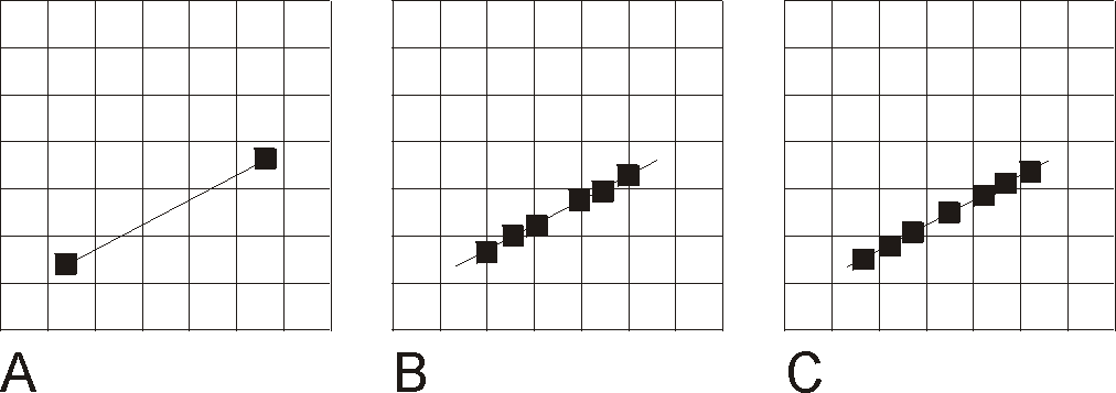 |
| Figure 2.5, Progressive steps in intersection of Polyline with grid cells. A. Line with endpoints. B. Intersection of line with row and column boundaries. C. Centers of segments used to determine cells intersected by the line. |
When the UpToDate property of TObserver is set to False, it notifies all TObservers that are talks to it. They set their own UpToDate property to False and continue the chain. If a TDataArray is out of date, it will recalculate its values the next time its values are needed.
ModelMuse allows the user to specify the values of data sets (see TDataArray) using formulas that calculate values based on the values of other data sets. Thus, when the value of one data set change, the values of other data sets may need to be recalculated.
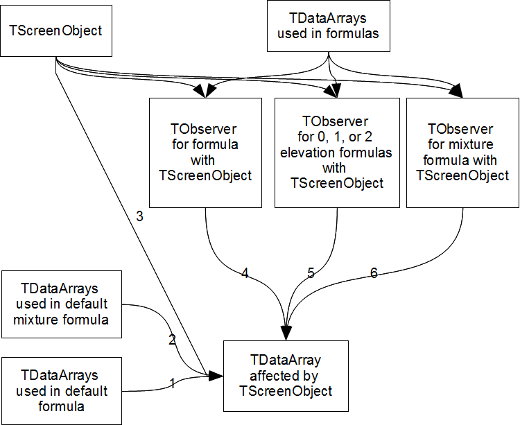
Each TDataArray talks to a series of other TObservers that affect it (figure 3.1). (1) Each is talks to the other TDataArrays that are used in its default formula. (2) If the TDataArray is a TCustomPhastDataSet, it may also have a mixture formula. The data set also talks to TDataArrays used in the mixture formula. (3) A TDataArray can have some of its values set by a TScreenObject. The TDataArray listens to the TScreenObject (4) as well as to a TObserver for the formula for the TScreenObject. (5) There may also be zero, one, or two elevation formulas. (See ElevationFunction, HigherElevationFunction, and LowerElevationFunction.) These are also represented by TObservers to which the TDataArray is listens. (6) In PHAST models, TScreenObject allows the specification of mixture formulas. Like the other formulas, these are represented by TObservers to which the TDataArray is listening.
The TObservers for the formulas associated with a TScreenObject talk to the TScreenObject as well as to the TDataArrays used in the formulas.
 |
| Figure 3.1, Notification network for TDataArray. |
Several components were developed as part of developing ModelMuse. Some of them probably would not be useful except in a program very similar to ModelMuse. Others have a wider applicability. These components are listed below.
Each dialog box has a Help button which when pressed will display the help for that dialog box.
Near the beginning of help for each dialog box is a description of how to display the dialog box. This is because the user may reach the help for the dialog box without having pressed the help button on that dialog box.
The help describes the function of each control on the dialog box in a logical order.
The names of dialog boxes, controls, menu items, and other textual elements not directly set by the user are displayed in a bold font when in the body but not if they are in a heading. For example: "the OK button." (In tables, the bold font may be omitted if the only thing in the table cell is the name.)
The user "clicks" on a button in a dialog box with the mouse but "presses" a button on the keyboard with his finger.
The names of dialog boxes and tabs are in Title Case.
The names of edit boxes, radio buttons, etc are in Sentence case.
Help Generator is a program for generating documentation for programs written in Object Pascal based on comments in the source code. Help Generator uses PasDoc (http://pasdoc.sipsolutions.net/FrontPage), an open-source Object-Pascal program and component to read the source code, extract the comments from it and format the comments as either a series of linked web pages or a LaTeX file. The LaTeX file can be easily converted into either a PostScript, Portable Document Format (PDF), or DVI file. The source code for Help Generator is available for download at the same location as ModelMuse.
Most of the source code for ModelMuse includes comments that can be used by Help Generator. However, ModelMuse includes some source code written by others and these files do not contain comments that can be used by Help Generator. The source code for Help Generator also includes a project file that can be used to set the options used by Help Generator to create documentation for ModelMuse. The project file only includes the names of source code files that include comments that can be used by Help Generator. A PDF of the source code documentation generated by Help Generator is included with ModelMuse. The web page from which ModelMuse can be downloaded contains a link to the web pages generated by Help Generator for ModelMuse. Help Generator project files are also available for the custom components in ModelMuse.
Help Generator can work in conjunction with the GraphViz dot program (http://www.graphviz.org/) to create some summary diagrams that are used in the documentation. It also works in conjunction with GNU Aspell (http://aspell.sourceforge.net/) which performs spell checking. The location of the Aspell program must be available in the search $PATH.
ModelMuse Testing Tool (formerly known as GoPhast Testing Tool) is a tool designed to run ModelMuse automatically. It starts ModelMuse, instructs it to read a ModelMuse file and exports the transport input file for PHAST or the input files for MODFLOW and MODPATH. It then compares the newly exported files to a previously archived version. If the new and archived files have the same contents, ModelMuse is considered to have passed the test. If the files are not identical, ModelMuse is considered to have failed the test and the user is informed of the problem. The user must then determine whether the new or old versions of the file is correct. If the old version of the file is correct but not the new one, a bug has been introduced into ModelMuse. When the source code of ModelMuse is modified, such tests should be run to ensure that the changes have not caused unexpected changes in how ModelMuse works.
Only opening files and exporting model input files in ModelMuse can be tested by the ModelMuse Testing Tool. Other aspects of ModelMuse must be tested manually.